Fluid Pressure (pp. 45-50)
Course Website
Fluid statics deals with forces in fluids that are have no relative motion within the fluid. The vessel containing the fluid may be at non-zero velocity or acceleration, but the fluid body within the vessel has no relative motion.
Readings
Hibbeler, R.C, Fluid Mechanics, 2ed. Prentice Hall, 2018. ISBN: 9780134655413 pp. 47-80
Cleveland, T. G. (2014) Fluid Mechanics Notes to Accompany CE 3305 at Jade-Holshule (TTU Study Abroad 2015-2019), Department of Civil, Environmental, and Construction Engineering, Whitacre College of Engineering. http://54.243.252.9/ce-3305-webroot/3-Readings/ce3305-lecture-003.1.pdf
DF Elger, BC Williams, Crowe, CT and JA Roberson, Engineering Fluid Mechanics 10th edition, John Wiley & Sons, Inc., 2013. Chapter 3 http://54.243.252.9/ce-3305-webroot/3-Readings/EFM-3.pdf
Videos
Lesson Outline
Shear and Normal Stress
Hydrostatic Equation (Pascal’s law)
Measuring Devices (Pressure)
Manometers (application of Pascal’s law)
Stress (pp. 20)
Fluid statics deals with forces in fluids that are have no relative motion within the fluid. The vessel containing the fluid may be at non-zero velocity or acceleration, but the fluid body within the vessel has no relative motion.
Two principal types of forces involved are body and surface forces as shown in Fig. 35
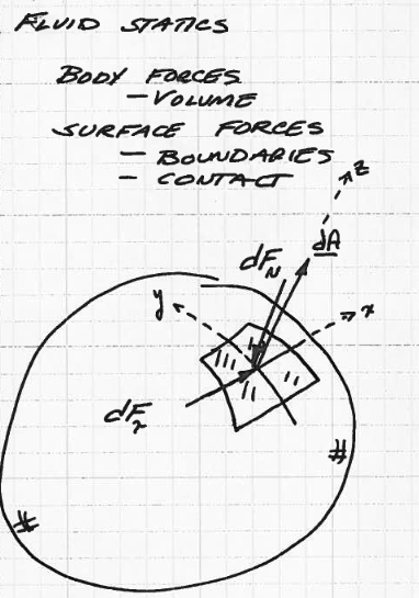
Fig. 35 A sphere of some fluid, depicting a local coordinate system, differential area and a normal and tangential force pair
Body forces are developed without contact and are distributed over the entire volume of a fluid. In the sketch the weight of the sphere is a body force.
Surface forces act at boundaries of a medium through contant. The normal force in the sketch (which is the product of pressure and area) is a surface force, defined on the surface of the sphere.
Stress is the limiting value of \(\frac{dF}{dA}\); in the sketch there are two stresses: a normal stress (usually called pressure), and a tangential stress (usually called shear).
Shear stresses are formed by friction, no-slip assumption, and other practically occuring situations.
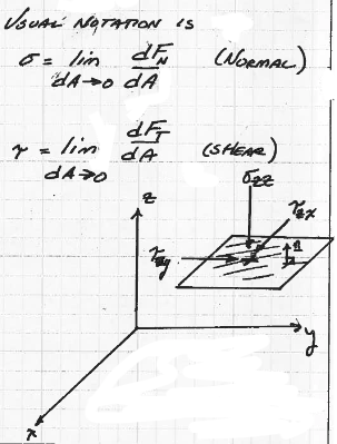
Fig. 36 Shear and normal stresses on a plane parallel to x-y coordinate plane, at some value z.
Fig. 36 is a diagram of a small planar element in a 3-D cartesian coordinate system that illustrate normal and shear stresses. The tensor-like naming system is also indicated.
A conventional notation is \(\sigma_{n,i-k}\) for normal stress, and \(\tau_{n,i-k}\) for shear stress. The first subscript is the direction of the outward pointing normal vector from the application plane (in the drawing +z), the second subscript is the direction of force application, with the normal stress positive into the plane. In the drawing the three stresses are \(\sigma_{z,z}\),\(\tau_{z,x}\), and \(\tau_{z,y}\).
Pressure (pp 45-51)
Fluid pressure (usual symbol \(p\)) is the normal stress applied to a fluid element, so in practice we simply make the direct substitution.
Note
The use of pressure in fluids and normal stress in solids is simply a convention - one could refer to solids pressure but that would confuse people.
Pressure is a normal force per unit area, so at any point within a fluid it is a scalar quantity. The dimensionality of pressure is the ratio of force to area; typical units are \(\frac{N}{m^2} = Pa\),\(\frac{lbs}{in^2}\). Pressure is also expressed in atmospheres \(1 atm = 101325Pa = 14.75psi\) and liquid column height \(1 atm \approx 10m_{water} \approx 29.92in_{Hg}\)
Note
Pressure is scalar (magnitude), the force it causes when pushing against an object is a vector (magnitude and direction)
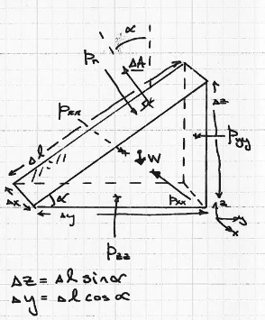
Fig. 37 FBD of small wedge of a static fluid.
Fig. 37 is a free body diagram of a small wedge of fluid; analyzing the wedge we can demonstrate that pressure is a scalar (Pascal’s Law).
First we will stipulate the fluid is a rest; no internal motion. Next perform a force balance in each direction as in Fig. 38
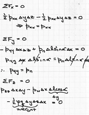
Fig. 38 Force balance x,y, and z directions on fluid wedge.
Notice we immediately invoke the definition of pressure to compute forces \(F=p \cdot A\) where \(A = \Delta x \Delta z\) and such, applying trigonometry to the wedge to resolve its force components. The directions are associated with the outward pointing normal vectors associated with the various planar areas.
We complete the analysis by studying the requirement of zero motion (statics) and find that indeed pressure is a scalar as in Fig. 39
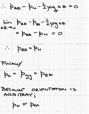
Fig. 39 Analysis summary and demonstration pressure must be scalar.
Because the three pressures are all the same at a point, we can drop the double subscript notation and simplify our notation herein.
Some practical application of Pascal’s Law is that in a closed system a change in pressure is transmitted undiminished throughout the entire system. This phenomenon is the basis of hydraulic machinery like pneumatic jacks (pg. 49 of the textbook)
Absolute and Gage Pressure (pp. 48-49)
Pressure is usually measured against some reference value. Two values in common use are a vaccum (zero pressure) and a standard atmosphere.
If the measurement is referenced to a standard atmosphere the measure is called gage pressure.
If the measurement is referenced to a vaccum, the measure is called absolute pressure
Gage pressures can be negative, but negative absolute pressures don’t make any sense.
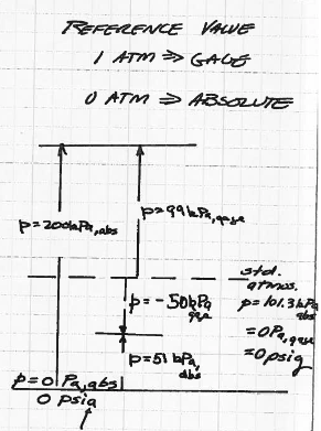
Fig. 40 Gage and absolute pressure.
Fig. 40 is a diagram depicting the relationship of gage and absolute pressures.
Hydrostatic Equation (pp. 50-52)
Here we develop the fundamental equation of fluid statics, and examine a couple of applications (pg. 52 is a condensed explaination).
Recall fluid statics means no relative motion within the fluid - the entire fluid behaves as a rigid body. The absence of angular deformation implies absence of shear stress; static fluids only sustain normal stress (pressure)
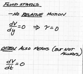
Fig. 41 Velocity gradient in static fluid
Fig. 41 is the mathematical statement of these stipulations.
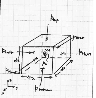
Fig. 42 Small fluid element in space (the final frontier!)
Consider a fluid element as in Fig. 42. We analyze the forces on the element taking limits as appropriate (continuum hypothesis) to recover the equation of a static fluid.
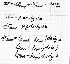
Fig. 43 Force balance statement, and naming of forces
Writing the surface and body forces of the element as a rigid body, and equating these forces to acceleration (Newton’s 2nd Law) produces a set of terms in Fig. 44
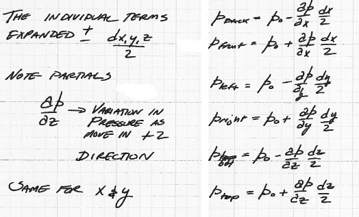
Fig. 44 Expansion of forces from centroid to front, back,left,right, top, bottom face of the small fluid element.
Using Taylor-series expansions about the centroid of the element
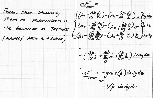
Fig. 45 Substitution into force definition (surface forces)
Fig. 45 is the substitution of our forces at each face into the equation of motion.
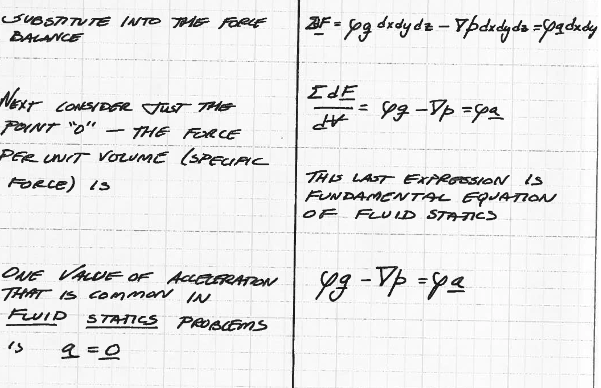
Fig. 46 Surface and body forces into balance equation; rescaling by element volume
Fig. 46 is the balance equation divided by the small but non-vanishing element volume to produce the fluid equation at an arbitrary point.
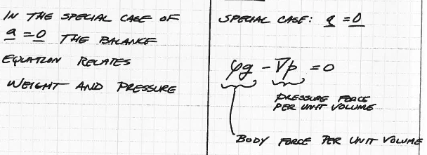
Fig. 47 Zero acceleration equation of fluid statics
Fig. 47 is the equation of motion (this is actually Euler’s equation - but he does not need it anymore!) at zero acceleration.
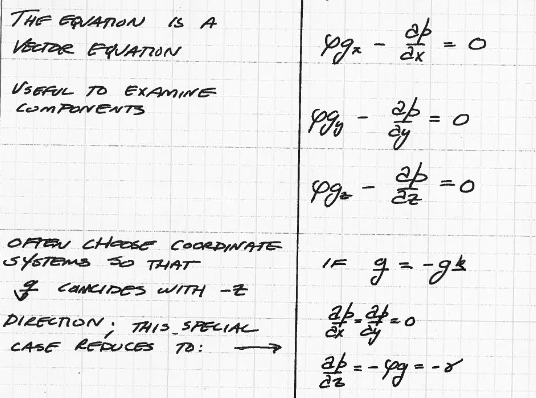
Fig. 48 Decomposition into cartesian components
Fig. 48 is the decomposition of the vector equation into its independent components, in this case cartesian coordinates. The \(z\)-axis equation is the only one conveying meaningful information (because of our choice of gravitational action).
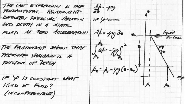
Fig. 49 Hydrostatic equation in a liquid
Fig. 49 is the hydrostatic equation for an incompressible liquid (like water). Pressure increases moving down from the free surface.
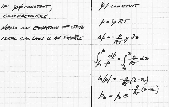
Fig. 50 Hydrostatic approximation for compressible fluid (like the atmosphere)
Fig. 50 is the hydrostatic approximation for compressible fluid. Here the ideal gas law is used as the equation of state.
Pressure Measurements (pp. 56 - 63)
Pressure is measured by a variety of devices depending on the fluid. Some of these are:
barometer (for measuring atmospheric pressure)
piezometer
manometer
Bourdon-type gages The principle of operation is the deformation of a curved tube in response to external pressure force change.
pressure transducers
Barometer
A barometer is a tube filled with liquid (oil,Hg,water), that is capped on one end, inverted into a basin and allowed to equilibrate as in Fig. 51
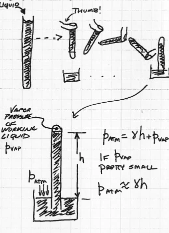
Fig. 51 Schematic of a barometer.
The height of rise is obtained from a force balance between the vapor pressure of the working fluid in the capped end and the surrounding atmospheric pressure.
Piezometer
A piezometer is a tube inserted into a fluid (usually liquid) which is open at both ends, large enough diameter so that capillary rise is negligible. The height of rise of liquid in the tube is proportional to the static pressure in the liquid at the bottom of the tube.
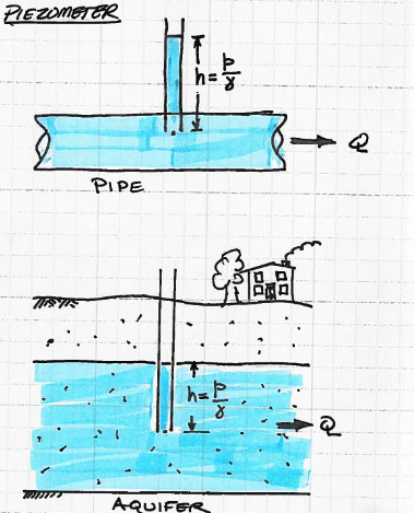
Fig. 52 Schematic of a piezometer.
A well in an aquifer is a common example of a piezometer that measures the water pressure at the bottom of the tube (or averaged over the well screen length)
Manometer
Manometers are like a hybrid of a barometer and piezometer.
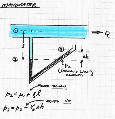
Fig. 53 Schematic of a manometer.
Manometers are connected to a fluid (measured), via an immiscible working fluid (usually oil or Hg). The force differential between the fluid and atmosphere is indicated by the working fluid.
As with similar devices the \(\frac{F}{A}\) is equated to the column height differential in the working fluid through \(h=\frac{p}{\rho_{w.f.}g}\)
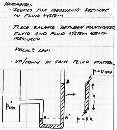
Fig. 54 Reading a manometer.
Multiple tube/fluid manometers follow 2 rules (Pascal’s law, and the hydrostatic equation)
Any two points at the same elevation in a continuous length of the same fluid are at the same pressure.
pressure increases with depth in a liquid column.
Transducers
[Insert link to sensor book here]
Examples
Below are a few examples applying the hydrostatic equation and Pascal’s law in a few different situations
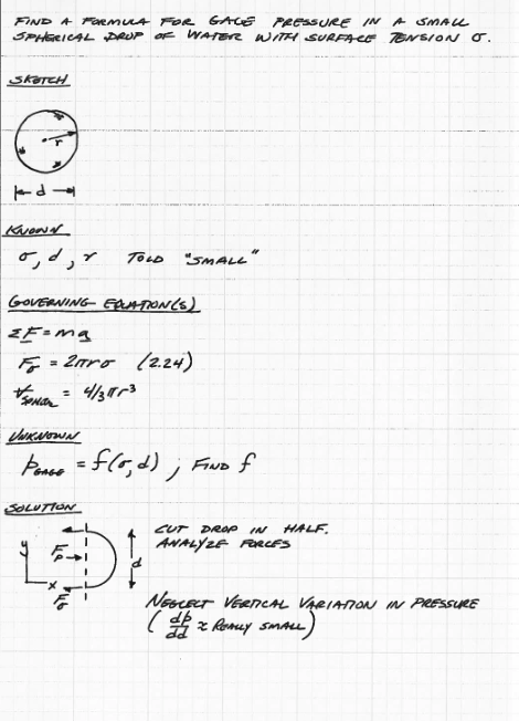
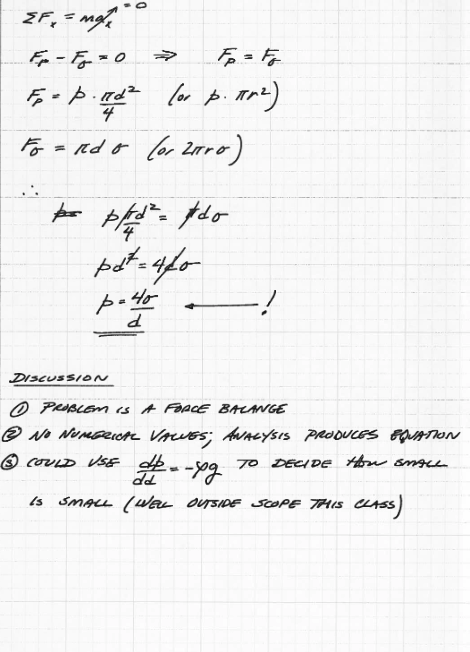
Example 1
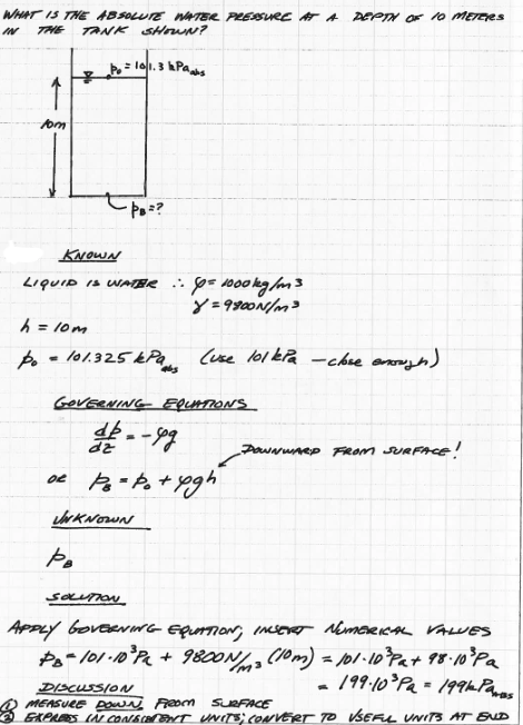
Fig. 55 Pressure at the bottom of a vessel.
Fig. 55 is a classical pressure at the bottom of a vessel, using the problem solving protocol.
Example 2
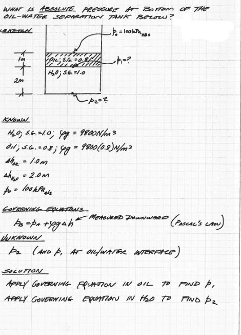
Fig. 56 Pressure in a two-layer fluid system (1 of 2)
Fig. 56 is an analysis of a multi-phase system (Air, Oil, Water), using the problem solving protocol.
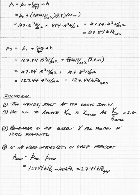
Fig. 57 Pressure in a two-layer fluid system (2 of 2)
Fig. 57 is an analysis of a multi-phase system (Air, Oil, Water), using the problem solving protocol.
Example 3
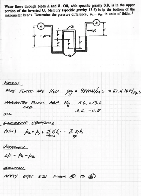
Fig. 58 Manometer with three fluids (1 of 3)
Fig. 58 is a manometer system, with two working fluids (and the measured fluid for three total)
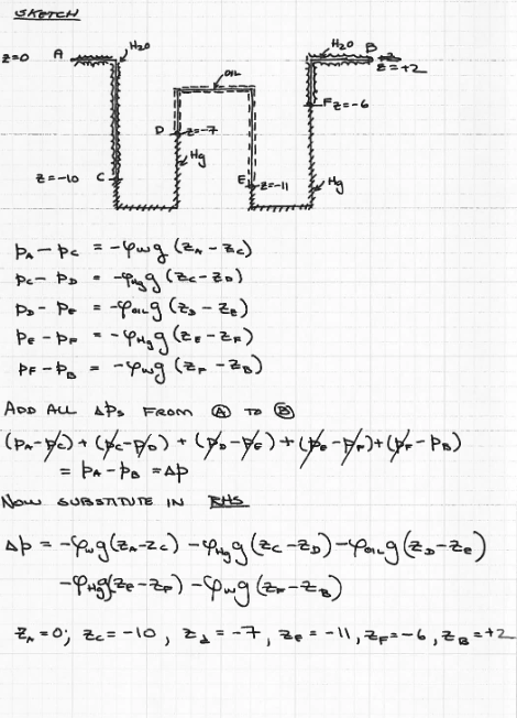
Fig. 59 Manometer with three fluids (2 of 3)
Fig. 59 is a manometer system, with two working fluids (and the measured fluid for three total)
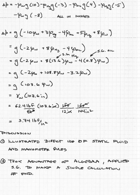
Fig. 60 Manometer with three fluids (3 of 3)
Fig. 60 is a manometer system, with two working fluids (and the measured fluid for three total)