Viscosity (pp 18-26)
“… a property of a fluid that relates the resistance to motion (in a thin layer) when a shear force is applied…”
This somewhat useless definition is trying to convey how fluids deform under shear, and more importantly the rate of deformation.
Consider a steel sheet that we cut with a shear (like sicssors), if we want to cut fast we need a lot of force; using the same shears on an equal thickness of plastic sheet will take less force for the same rate of cut.
This solids analog to viscosity conveys that steel is more viscous than plastic (usually).
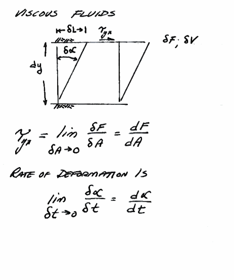
Fig. 11 Viscosity Schematic
Fig. 11 Is a diagram attempting to convey the concept of viscosity. In the drawing the thickness \(\partial y\) and the deformation angle \(\partial \alpha\) are small, and the sine of the angle is approximated by the angle itself.
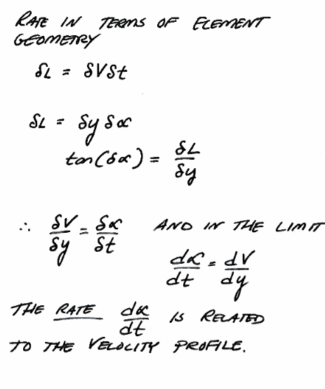
Fig. 12 Viscosity Trigonometry
Fig. 12 shows the relevant trigonometry to relate deformation rate to shear stress.
Absolute Viscosity
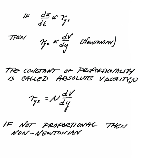
Fig. 13 Absolute viscosity (definition)
Fig. 13 defines a Newtonian fluid and introduces the absolute viscosity \(\mu\) in terms of the thin layer, cross-layer velocity profile \(\frac{du}{dy}\) and the applied shear stress \(\tau\). The viscosity has dimensions of \(\frac{Force \cdot Time}{Area}\)
Apparent Viscosity
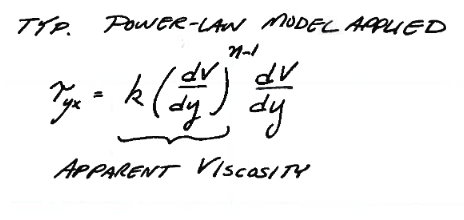
Fig. 14 Apparent viscosity (definition) power-law model
Fig. 14 shows a typical power-law model of viscosity; the term is referred to as an apparent viscosity. Many real fluids are Non-Newtonian and will have some type of viscosity model to explain the deformation behavior.
Kinematic Viscosity
The ratio of absolute (or apparent) viscosity to the fluid density is called the kinematic viscosity. The usual symbol is \(\nu = \frac{\mu}{\rho}\) The kinematic viscosity has dimensions of \(\frac{Area}{Time}\)
General Comments
Viscous effects cause a velocity gradient (profile) to develop across the fluid layers as shown in Fig. 15.
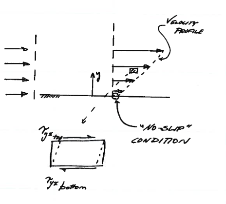
Fig. 15 Velocity Profile Diagram
Fig. 15 is a diagram of the cross-layer velocity profile. The slope of the profile is related to shear force and hence the apparent or absolute viscosity.
Note
The no-slip condition is deduced from experiments - in my opinion it is an assumption that velocity vanishes at the contact interface. In your future studies keep this in mind; it is quite possible that slip occurs at some scale, however it is a useful and accepted boundary condition.
Example 1
Here is a hand-worked example to illustrate viscosity concepts and problem solving protocol.
We start with a problem statement:

Fig. 16 Block sliding on an inclined plane
Fig. 16 is a problem statement of the problem we wish to solve.
The next step is to sketch the situation, mindful of several different scales in the problem.

Fig. 17 Block sliding on an inclined plane (various definining sketches)
Fig. 17 is a set of sketches, showing the macro-scale conditions, as well as a free-body-diagram, and a sketch of the fluid layer between the block and the plane.
Next we list knowns, unknowns, and governing equations:

Fig. 18 Known or given values
Fig. 18 is a list of known or supplied (in the problem statement) values

Fig. 19 Unknown (sought) values
Fig. 19 is a list of unknown or sought values

Fig. 20 Relevant equations
Fig. 20 is an initial list of applicable equations (we may add to this list as the analysis proceedes).
Now we proceede with the analysis
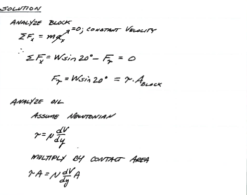
Fig. 21 Solution
Fig. 21 is our initial work towards a solution, ending with an expression relating shear force and viscosity.
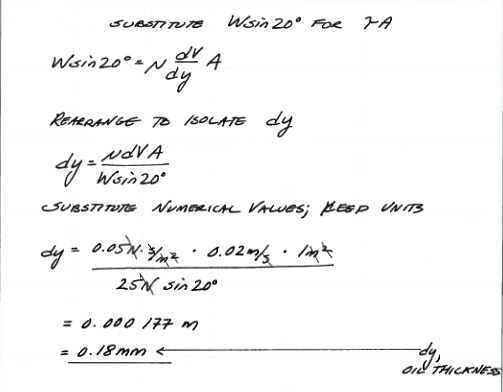
Fig. 22 Solution(continued)
Fig. 22 is the completion where the geomtric terms are inserted and a numerical answer is supplied.
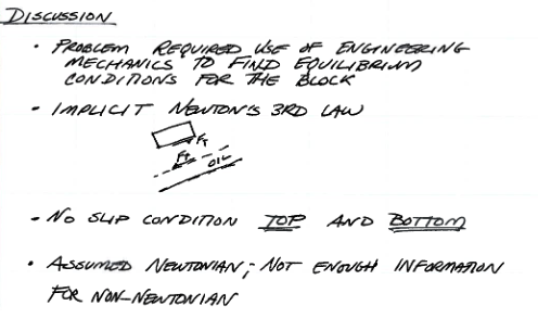
Fig. 23 Discussion of results
Fig. 23 is a discussion of results; this part is important as part of professional documentation, esp. if the analysis is a first approximation and is being used to determine whether further work will be needed.
Example 2 - Radial Geometry Kinematics
A similar example is presented below, however the geometry is changed a bit.
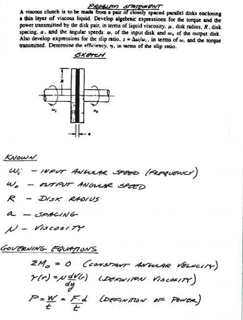
Fig. 24 Fluid drive problem (i.e how a transmission works!)
Fig. 24 is a problem statement and list of known values and governing equations.
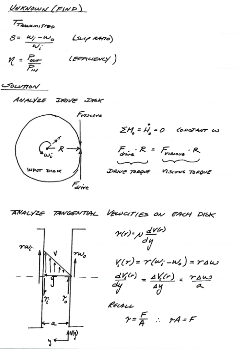
Fig. 25 Schematic sketches to define problem terms
Fig. 25 is a list of unknown values and defining sketches. Notice the geometry poses some complexity, hence the varied drawings to guide analysis.
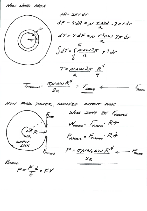
Fig. 26 Schematic sketches to define problem terms (continued)
Fig. 26 are continued defining sketches and associated analyses.
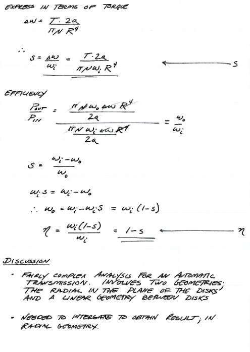
Fig. 27 Results and Discussion
Fig. 27 is the results in useful units, and a discussion of the findings. The problem parts are straightforward using concepts for prior classes, but the analyst does have to keep track of the steps to get to a useable solution.
Viscometers
A variety of instruments are used to measure viscosity.
They all operate on roughly the same principle - determine the force requires to make two solid planes move with a fluid between then; from the force and known geometry the viscosity can be inferred. The example problem below is a falling piston viscometer - with the question asked in an unusual fashion, but it could easily be used to measure viscosity based on a measured fall velocity.
Example Problem
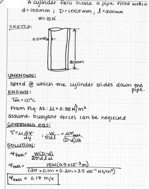
Figure Fig. 28 is a schematic of a cylinder falling inside a pipe that is filled with oil. The annular space between the cylinder and the pipe is lubricated with an oil film that has viscosity \(\mu\).
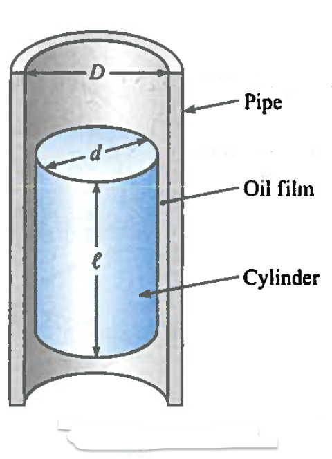
Fig. 28 Falling cylinder in an oil-filled pipe
Derive a formula for the steady rate of descent of a cylinder with weight \(W\) , diameter \(d\), and length \(l\) sliding inside a vertical smooth pipe that has inside diameter \(D\). Assume the cylinder remains concentric with the pipe as it falls.
Use the general formula you develop to estimate the rate of descent for a cylinder 100 millimeters in diameter that slides inside a 100.5 millimeter inside diameter pipe. The cylinder is 200 millimeters long and weighs 15 Newtons. The lubricant is SAE 20W oil at \(10^o~C\).
Applying the problem solving methodology we have:
We can easily script a tool for frequent application of a falling cylinder viscometer
# falling piston viscometer
import math
# viscosity function for falling piston in a tube geometry
def viscosity(weight,spacing,dpiston,lpiston,velocity):
    viscosity = (weight*spacing)/(2*math.pi*dpiston*lpiston*velocity)
    return viscosity
# Example Problem Values
weight = 15 #newtons
spacing = 0.5e-03 #meters spacing
dpiston = 0.1 #meters
lpiston = 0.2 #meters
velocity = 0.17 #meters/sec
print("Viscosity = ",round(viscosity(weight,spacing,dpiston,lpiston,velocity),3)," Newtons per square meter")
Viscosity = 0.351 Newtons per square meter

