Example Applications of Continunity (pp. 182)
Example 1: Application of Continunity to a Spa
Consider an open tank with two connections as depicted in Fig. 92
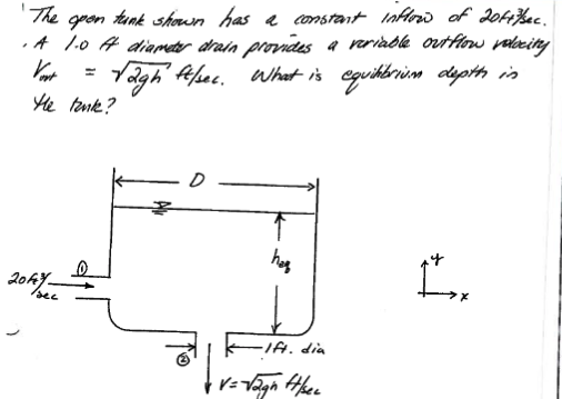
Fig. 92 Open tank with inlet and outlet
Apply our problem solving protocol as in Fig. 93
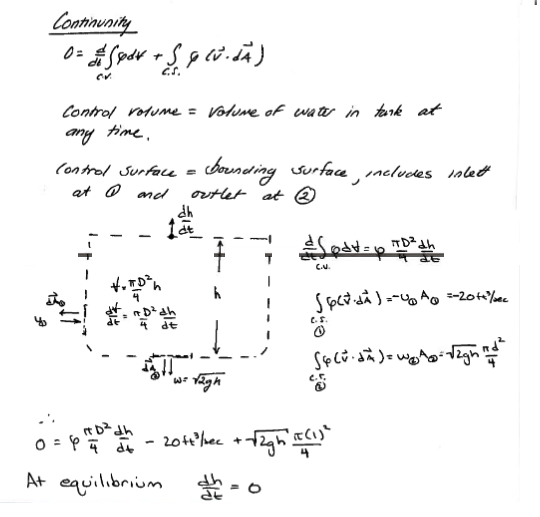
Fig. 93 Problem Solving Protocol: Sketch, CV Definition, Governing Principles, Knowns and Unknowns
Once we have a formula we can use ENGR-1330 tools (as a calculator):
import math
# known
Q_in = 20 # cuft/s
D_out = 1.0 # m^2
gravity = 32.2 # ft/s/s
# intermediate
A_out = math.pi*pow(D_out,2)/4.0
# equilibrium depth
h = pow(Q_in/A_out,2)/(2*gravity)
print('equilibrium depth is .... wait for it ...',round(h,1),'feat')
equilibrium depth is .... wait for it ... 10.1 feat
Example 2: Time to Drain a Tank
Consider an open tank as depicted in Fig. 94
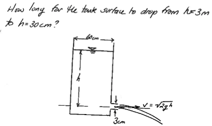
Fig. 94 Open tank with outlet
Apply our problem solving protocol as in Fig. 95
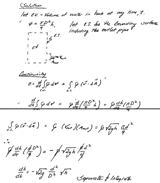
Fig. 95 Problem Solving Protocol: Sketch, CV Definition, Governing Principles, Knowns and Unknowns
Apply our Calculus tools from MATH 2450
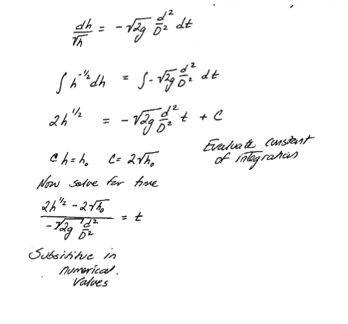
Fig. 96 Separation and Integration
Once we have a formula we can use ENGR-1330 tools (as a calculator):
import math
H_0 = 3    # meters initial depth
H   = 0.3  # meters ending depth
D   = 0.6  # meters tank diameter
d   = 0.03 # meters outlet diameter
g   = 9.8  # m/s/s gravitational avcceleeration conastant
# calculations
time = (2*math.sqrt(H)-2*math.sqrt(H_0)) / -(math.sqrt(2*g)*pow(d/D,2))
print('Time to drain is',round(time,1),'seconds')
Time to drain is 214.0 seconds
Example 3: Time to Drain a Tank
Now consider a similar problem
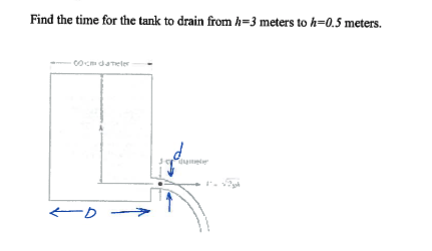
Fig. 97 Open tank with outlet
We can inspect and establish that it is an identical situation with different diameters of the tank and hole, and different starting and ending depths, so we can use our tool just developed.
import math
H_0 = 3    # meters initial depth
H   = 0.5  # meters ending depth
D   = 0.6  # meters tank diameter
d   = 0.03 # meters outlet diameter
g   = 9.8  # m/s/s gravitational acceleration conastant
# calculations
time = (2*math.sqrt(H)-2*math.sqrt(H_0)) / -(math.sqrt(2*g)*pow(d/D,2))
print('Time to drain is',round(time,1),'seconds')
Time to drain is 185.2 seconds
Example 4: Time to Drain a Tank (Computational Methods)
Now consider a pressure tank with oil
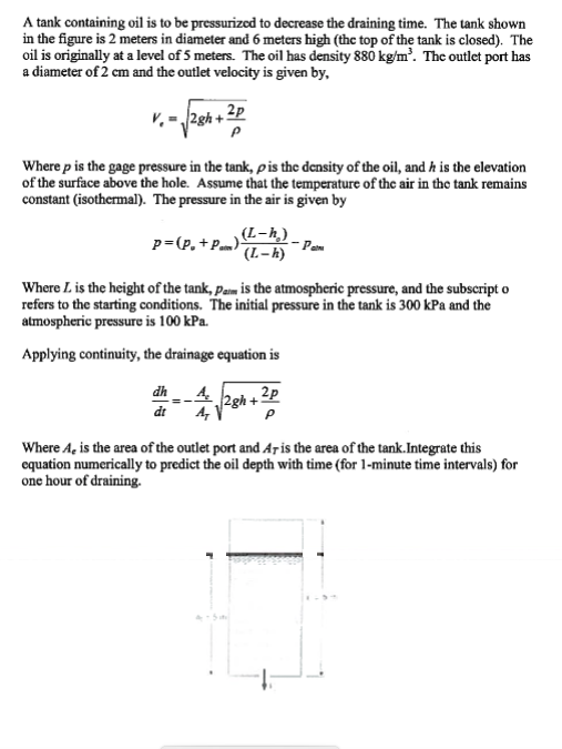
Fig. 98 Pressure tank with outlet
Here we are given the drainage equation, and the variable pressure terms, but cannot apply analysis (Calculus) to obtain a closed-form solution, thus we can:
Give up
Practice saying “How about a hot apple pie to go with that slop?”
Approximate using ENGR-1330 tools
Simply insert the pressure term into the drainage equation and develop a function to estimate the change in eleveation over a short time as:
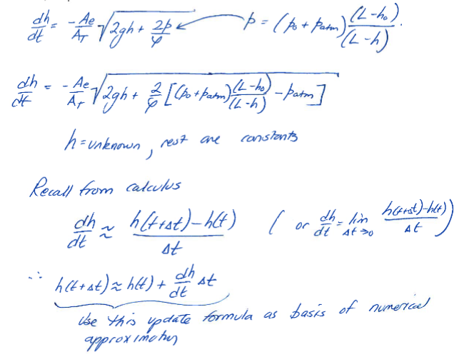
Fig. 99 Pressure tank with outlet
Now we can build a tool
import math
import matplotlib.pyplot as plt
# a plotting function
def make2plot(listx1,listy1,listx2,listy2,strlablx,strlably,strtitle):
    mydata = plt.figure(figsize = (10,5)) # build a square drawing canvass from figure class
    plt.plot(listx1,listy1, c='red', marker='v',linewidth=0) # basic data plot
    plt.plot(listx2,listy2, c='blue',linewidth=1) # basic model plot
    plt.xlabel(strlablx)
    plt.ylabel(strlably)
    plt.legend(['Tank Level',''])# modify for argument insertion
    plt.title(strtitle)
    plt.show()
    return
# constants
pie = math.pi
p_initial = 3e05 #Pa initial pressure
p_atm     = 1.01e05 #Pa atmospheric pressure
g         = 9.8  #m/s/s
rho_oil   = 1000 #kg/m^3
L         = 6    #m tank height
De        = 0.02 #m outlet diameter
Dt        = 2.0  #m tank diameter
H0        = 5    #m initial depth
time      = []   # time seconds, an empty list
depth     = []   # depth meters, an empty list
pnow      = []   # pressure, an empty list
ddepth    = []   #change in depth, empty list for debuggiun'
how_many  = 60   #time steps
deltat    = 60   #seconds a time step length
# constants
Ae = (pie*De**2)/4
At = (pie*Dt**2)/4
# pressure function
def p_now(p_initial,p_atm,L,H0,H):
    p_now = (p_initial+p_atm)*((L-H0)/(L-H))#-p_atm
    return(p_now)
# CV velocity function
def dhdt(Ae,At,g,H,p,rho):
    dhdt = -(Ae/At)*math.sqrt(2*g*h + 2*p/rho)
    return(dhdt)
# initial conditions
time.append(0)
depth.append(H0)
pnow.append(p_initial)
ddepth.append(dhdt(Ae,At,g,H0,p_now(p_initial,p_atm,L,H0,H0),rho_oil))

for i in range(1,how_many):
    time.append(i*deltat)
    depth.append(depth[i-1]+deltat*ddepth[i-1])
    if depth[i] < 0:
        depth[i]=0.0
    pnow.append(p_now(p_initial,p_atm,L,H0,depth[i]));
    ddepth.append(dhdt(Ae,At,g,depth[i],pnow[i],rho_oil))


#for i in range(how_many):
#    print(time[i],round(depth[i],3),round(pnow[i],3),round(ddepth[i],6))

#now plot
make2plot(time,depth,time,depth,'Time(sec)',"Depth(m)","Tank oil level")
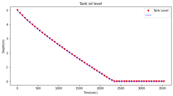
While not at all perfect it illustrates using a computational method to approximate the problem, and more importantly determine a good guess of the time to drain the tank.
