
ENGR 1330 Computational Thinking with Data Science
Copyright © 2021 Theodore G. Cleveland and Farhang Forghanparast
Last GitHub Commit Date:
9: Matrix Manipulation(s) using NumPy
How to install
conda
pip in JupyterHub/Lab (on Linux)
About NumPy
Arrays
Array Methods
Examples using NumPy to illustrate abstraction to maintainable scripts
Objectives
To understand the representation of data in different structure using the NumPy library(module).
Access data within a NumPy array
Perform arithmetic/mathematical operations on the contents of NumPy arrays
Numpy
Numpy is the core library for scientific computing in Python. It provides a high-performance multidimensional array object, and tools for working with these arrays. The library’s name is short for “Numeric Python” or “Numerical Python”. If you are curious about NumPy, this cheat sheet is recommended: https://s3.amazonaws.com/assets.datacamp.com/blog_assets/Numpy_Python_Cheat_Sheet.pdf
NumPy library has two fundamental conceptualizations:
Data representation: Arrays
vectors
matrices
Data operations:
Element-by-element arithmetic, and mathematical operations;
Matrix/vector arithmetic
Indexing
Selection
Copying
Computational Thinking Concepts
The CT concepts expressed within NumPy include:
Decomposition: Break a problem down into smaller pieces; Data interpretation, manipulation, and analysis of NumPy arrays is an act of decomposition.Abstraction: Pulling out specific differences to make one solution work for multiple problems; The array is a data representation abstraction that allows for placeholder operations, later substituted with specific contents for a problem; enhances reuse and readability. Generally we leverage the principle of algebraic replacement using these abstractions.Algorithms: A list of steps that you can follow to finish a task; Data interpretation, manipulation, and analysis of NumPy arrays is generally implemented as part of a supervisory algorithm.
Module Set-Up
In principle, NumPy should be available in a default Anaconda install
You should not have to do any extra installation steps to install the library in Python
You do have to import the library in your scripts
How to check
Simply open a code cell and run
import numpyif the notebook does not protest (i.e. pink block of error), you is good to go.
import numpy
If you do get an error, that means that you will probably have to install using conda or pip; generally this process of installation is only needed occassionally, you are installing into your kernel the needed funcrtionality.
Note
On the content server the process is:
Open a new terminal from the launcher
Change to root user
suthen enter the root passwordsudo -H /opt/jupyterhib/bin/python3 -m pip install numpyWait until the install is complete; for security, user
compthinkis not in thesudogroupVerify the install by trying to execute
import numpyas above.
The process will be similar on a Macintosh, or Windows. Best is to hope you have a sucessful anaconda install.
If you have to do this kind of install, you will have to do some reading, some references I find useful are:
https://jupyterlab.readthedocs.io/en/stable/user/extensions.html
https://jupyterhub.readthedocs.io/en/stable/installation-guide-hard.html (This is the approach on the content server which has a functioning JupyterHub)
Note
The conda installer is accessed using the conda powershell prompt, accessed from Anaconda Navigator.
Here are some useful videos:
NumPy: AKA Numerical Python
NumPy is a foundational library (module) for scientific computing. Most if not all all data science libraries (modules) rely on NumPy as one of their building blocks to reduce the need to build certain operations in primative python.
NumPy provides a multi-dimensional array object called ‘ndarray’ (n-dimensional array) and methods for:
Computations with arrays and mathematical operations between arrays (array-by-array and element-by-element)
Linear algebra operations
Psuedo random number generation
As compared to the prior lesson, multi-dimensional arrays (lists) are far easier to manipulate using numpy.
Arrays
A numpy array is a grid of values, all of the same type, and is indexed by a tuple of nonnegative integers. The number of dimensions is the rank of the array; the shape of an array is a tuple of integers giving the size of the array along each dimension.
The figure below is a visual depiction of numpy arrays of rank 1 and rank2.
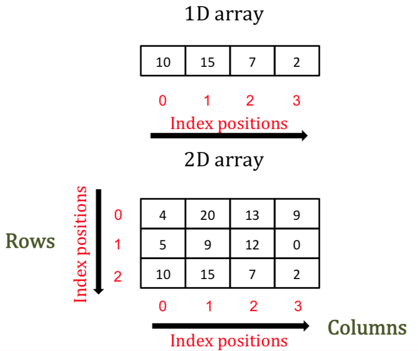
In other words, an array contains information about the raw data, how to locate an element and how to interpret an element.To make a numpy array, you can just use the np.array() function. All you need to do is pass a list to it. Don’t forget that, in order to work with the np.array() function, you need to make sure that the numpy library is present in your environment.
If you want to read more about the differences between a Python list and NumPy array, this link is recommended:
https://webcourses.ucf.edu/courses/1249560/pages/python-lists-vs-numpy-arrays-what-is-the-difference
Example- 1D Arrays (Vectors)
Let’s create a 1D array from the 2000s (2000-2009):
import numpy             #First, we need to impoty "numpy"
mylist = [2000,2001,2002,2003,2004,2005,2006,2007,2008,2009]         #Create a list of the years
type(mylist)
list
print(mylist) #Check how it looks
[2000, 2001, 2002, 2003, 2004, 2005, 2006, 2007, 2008, 2009]
mylist = numpy.array(mylist)              #Type cast it as a numpy array
type(mylist)
numpy.ndarray
print(mylist)
[2000 2001 2002 2003 2004 2005 2006 2007 2008 2009]
my2dlist = [[1,2,3],[4,5,6],[7,8,9]]
type(my2dlist)
list
print(my2dlist)
[[1, 2, 3], [4, 5, 6], [7, 8, 9]]
my2dlist= numpy.array(my2dlist)   #Type cast it as a numpy array
type(mylist)
numpy.ndarray
print(my2dlist)
[[1 2 3]
 [4 5 6]
 [7 8 9]]
len(my2dlist) #how many rows
3
len(my2dlist[0]) #how many columns
3
numpy.shape(my2dlist) # using the shape method
(3, 3)
Example: n-Dimensional Arrays
We already made a 3X3 array, but let’s create a 5x2 array from the 2000s (2000-2009):
myotherlist = [[2000,2001],[2002,2003],[2004,2005],[2006,2007],[2008,2009]]     #Since I want a 5x2 array, I should group the years two by two
print(myotherlist)             #See how it looks as a list
print(numpy.shape(myotherlist)) #check the shape
print(numpy.array(myotherlist)   )       #See how it looks as a numpy array
[[2000, 2001], [2002, 2003], [2004, 2005], [2006, 2007], [2008, 2009]]
(5, 2)
[[2000 2001]
 [2002 2003]
 [2004 2005]
 [2006 2007]
 [2008 2009]]
Array Arithmetic
Once you have created the arrays, you can do basic Numpy operations. Numpy offers a variety of operations applicable on arrays. From basic operations such as summation, subtraction, multiplication and division to more advanced and essential operations such as matrix multiplication and other elementwise operations. In the examples below, we will go over some of these:
Example- 1D Array Arithmetic
Define a 1D array with [0,12,24,36,48,60,72,84,96]
Lets do scalar multiplication, first as just a list!
# interactive cell - copy/paste into a notebook to run
victorVector = [0,12,24,36,48,60,72,84,96]
MyScalar = input("Enter scalar value \n")
MyScalar = float(MyScalar)  # force a float
# now perform element-by-element multiplication
for i in range(0,len(victorVector),1):
    victorVector[i] = MyScalar * victorVector[i] # this will change contents of amatrix
print(victorVector)
Now using numpy
import numpy         #import numpy
Array1 = numpy.array([0,12,24,36,48,60,72,84,96])     #Step1: Define Array1
print(Array1)
[ 0 12 24 36 48 60 72 84 96]
Multiply all elements by scalar value (scalar multiplication), print result, leave array unchanged
# interactive cell - cut/paste into a notebook to run
MyScalar = input("Enter scalar value \n")
MyScalar = float(MyScalar)  # force a float
# now perform element-by-element multiplication
print(Array1*MyScalar)     #Step2: Multiple all elements by 2
Take all elements to the power of 2
print(Array1**2) #Step3: Take all elements to the power of 2
[ 0 144 576 1296 2304 3600 5184 7056 9216]
print(numpy.power(Array1,2)) #Another way to do the same thing, by using a function in numpy
[ 0 144 576 1296 2304 3600 5184 7056 9216]
Find the maximum value of the array and its position
print(numpy.max(Array1)) #Step4: Find the maximum value of the array
96
print(numpy.argmax(Array1)) ##Step4: Find the postition of the maximum value
8
Find the minimum value of the array and its position
print(numpy.min(Array1)) #Step5: Find the minimum value of the array
0
print(numpy.argmin(Array1)) ##Step5: Find the postition of the minimum value
0
Define another 1D array with [-12,0,12,24,36,48,60,72,84]
Array2 = numpy.array([-12,0,12,24,36,48,60,72,84])     #Step6: Define Array2
print(Array2)
[-12 0 12 24 36 48 60 72 84]
Find the element-by-element sum and difference of these two arrays
print(Array1+Array2)         #Step7: Sum of two arrays
print(Array1-Array2)         #Step7: Difference of two arrays
[-12  12  36  60  84 108 132 156 180]
[12 12 12 12 12 12 12 12 12]
Element-by-element multiplication of these two arrays
print(Array1*Array2) #Step8: Find the multiplication of these two arrays
[ 0 0 288 864 1728 2880 4320 6048 8064]
Example- n-Dimensional Array Arithmetic
Define a 2x2 array with [5,10,15,20]
import numpy         #import numpy
Array1 = numpy.array([[5,10],[15,20]])     #Step1: Define Array1
print(Array1)
[[ 5 10]
 [15 20]]
Define another 2x2 array with [3,6,9,12]
Array2 = numpy.array([[3,6],[9,12]])     #Step2: Define Array2
print(Array2)
[[ 3  6]
 [ 9 12]]
Find the sum and difference of these two arrays
print(Array1+Array2)     #Step3: Find the summation
print(Array1-Array2)     #Step3: Find the subtraction
[[ 8 16]
 [24 32]]
[[2 4]
 [6 8]]
Find the minimum number in the multiplication of these two arrays
MultArray = Array1@Array2         #Step4: To perform a typical matrix multiplication (or matrix product)
print(MultArray)
MultArray1 = Array1.dot(Array2)         #Step4: Another way To perform a  matrix multiplication
print(MultArray1)
print(numpy.min(MultArray))     #Step4: Find the minimum value of the multiplication
[[105 150]
 [225 330]]
[[105 150]
 [225 330]]
105
Recall how we have to do the same if using ordinary lists, just for the first line in the block above:
amatrix = [[5,10],[15,20]]
bmatrix = [[3,6],[9,12]]
cmatrix = [[0 for j in range(len(bmatrix[0]))] for i in range(len(amatrix))] # 2D list to receive input; explicit sizing
# now for the multiplication
for i in range(0,len(amatrix)):
    for j in range(0,len(bmatrix[0])):
        for k in range(0,len(amatrix[0])):
            cmatrix[i][j]=cmatrix[i][j]+amatrix[i][k]*bmatrix[k][j]
for i in range(len(cmatrix)): # print by row
    print(cmatrix[i][:])
[105, 150]
[225, 330]
There is considerable savings in code crafting using numpy; hence its popularity and utility.
Find the position of the maximum in the multiplication of these two arrays
print(numpy.argmax(MultArray)) ##Step5: Find the postition of the maximum value
3
Find the mean of the multiplication of these two arrays
Find the mean of the first row of the multiplication of these two arrays
print(numpy.mean(MultArray))     ##Step6: Find the mean of the multiplication of these two arrays
print(numpy.mean(MultArray[0,:]))     ##Step7: Find the mean of the first row of the multiplication of these two arrays
202.5
127.5
Other functions to create NumPy arrays easily
arange( ): Returns evenly spaced array elementslinspace( ): Returns evenly spaced array elementszeros( ): Returns an array of zerosones( ): Returns an array of onesrandom.randint(.): Returns random integers
Functions to do basic operations on NumPy arrays
min( ): Returns minimum value in an arraymax( ): Returns maximum value in an arrayargmin( ): Returns minimum value position in an arrayargmax( ): Returns maximum value position in an arrayreshape( ): Reshaping an array to a specific shapesort( ): Sorting an array in ascending ordersum( ): Summing the array elements (Demo)
Functions to do mathematical operations on NumPy arrays
sqrt( ): Returns square root of array elementsexp( ): Returns exponential of array elementssin( ): Returns trigonometric sine of array elementscos( ): Returns trigonometric cosine of array elementslog( ): Returns natural logarithm of array elementslog10( ): Returns base 10 logarithm of array elements
Indexing: An important step in manipulating and analyzing arrays
Conditional selection: Selecting array elements based on specific conditions typed using conditional operators
Copying: Use the copy( ) function to copy arrays and to preserve the original array
There are linear algebra functions too, recall our matrices
We can get the inverse in numpy from:
amatrix = [[2 ,  3 ],  # a and b are inverses of each other.
           [4 , -3 ]]
bmatrix = [[1/6 , 1/6 ],
           [2/9 , -1/9]]  # if we invert b should get a back.
amatrix = numpy.array(amatrix) # type cast to numpy arrays
bmatrix = numpy.array(bmatrix)
print(amatrix@bmatrix) # proof of inverse - should get identity
print(numpy.linalg.inv(bmatrix)) # invert b, see if we get a  - sho 'nuff
[[1. 0.]
 [0. 1.]]
[[ 2.  3.]
 [ 4. -3.]]
Arrays Comparison
Comparing two NumPy arrays determines whether they are equivalent by checking if every element at each corresponding index are the same.
Example- 1D Array Comparison
Define a 1D array with [1.0,2.5,3.4,7,7]
Define another 1D array with [5.0/5.0,5.0/2,6.8/2,21/3,14/2]
Compare and see if the two arrays are equal
Define another 1D array with [6,1.4,2.2,7.5,7]
Compare and see if the first array is greater than or equal to the third array
import numpy          #import numpy
Array1 = numpy.array([1.0,2.5,3.4,7,7])     #Step1: Define Array1
print(Array1)
Array2 = numpy.array([5.0/5.0,5.0/2,6.8/2,21/3,14/2])     #Step2: Define Array1
print(Array2)
print(numpy.equal(Array1, Array2))             #Step3: Compare and see if the two arrays are equal
Array3 = numpy.array([6,1.4,2.2,7.5,7])     #Step4: Define Array3
print(Array3)
print(numpy.greater_equal(Array1, Array3))             #Step3: Compare and see if the two arrays are equal
[1.  2.5 3.4 7.  7. ]
[1.  2.5 3.4 7.  7. ]
[ True  True  True  True  True]
[6.  1.4 2.2 7.5 7. ]
[False  True  True False  True]
Example n-Dimensional Array Comparison
Using the numbers below:
4,9,23,39,40,55,68,72
Create a 2x2 array with all the even numbers and print it out
Create a 2x2 array with all the odd numbers and print it out
Compare the two arrays using the “less_equal” function from numpy package
import numpy          #import numpy
Array1 = numpy.array([[4,40],[68,72]])     #Step1: Define Array1
print(Array1)
Array2 = numpy.array([[9,23],[39,55]])     #Step2: Define Array2
print(Array2)
print(numpy.less_equal(Array1,Array2))
[[ 4 40]
 [68 72]]
[[ 9 23]
 [39 55]]
[[ True False]
 [False False]]
Arrays Manipulation
numpy.copy() allows us to create a copy of an array. This method is particularly useful when we need to manipulate an array while keeping an original copy in memory.
The numpy.delete() function returns a new array with sub-arrays along an axis deleted. Let’s have a look at the examples.
Examples: Copying and Deleting Arrays and Elements
Below we will work a few examples.
Define a 1D array, named “x” with [1,2,3]
import numpy          #import numpy
x = numpy.array([1,2,3])     #Step1: Define x
print(x)
[1 2 3]
Assign “y” so that “y=x”
y = x                     #Step2: Assign y as y=x
print(y)
[1 2 3]
Define “z” as a copy of “x”
z = numpy.copy(x)    #Step3: Define z as a copy of x
print(z)
[1 2 3]
Discuss the difference between y and z
print('x = ',x)  # They look similar but ...
print('y = ',y)
print('z = ',z)
x =  [1 2 3]
y =  [1 2 3]
z =  [1 2 3]
now lets change a value in x, then print the contents again
x[0] = 100
print('x = ',x)  # For Step4: They look similar but ...
print('y = ',y)
print('z = ',z)
x =  [100   2   3]
y =  [100   2   3]
z =  [1 2 3]
Notice how x and y reflect the change, whats going on? The assignment statement y = x creates equivalence in numpy; that is x and y are different names for the same object. We can verify using the id() function which will return the address in memory of the head of the object.
print(' x object at hex address ',hex(id(x)))
print(' y object at hex address ',hex(id(y)))
print(' z object at hex address ',hex(id(z)))
 x object at hex address  0xffff6d9c1ee0
 y object at hex address  0xffff6d9c1ee0
 z object at hex address  0xffff6d9b8260
Delete the second element of x
x = numpy.delete(x, 1)      #Step5: Delete the second element of x, remember counting starts at zero
print('x = ',x)  # For Step4: They look similar but ...
print('y = ',y)
print('z = ',z)
x =  [100   3]
y =  [100   2   3]
z =  [1 2 3]
print(' x object at hex address ',hex(id(x))) # lets check the objects - now they are all different
print(' y object at hex address ',hex(id(y)))
print(' z object at hex address ',hex(id(z)))
 x object at hex address  0xffff6d9c18f0
 y object at hex address  0xffff6d9c1ee0
 z object at hex address  0xffff6d9b8260
Sorting Arrays
Sorting means putting elements in an ordered sequence. Ordered sequence is any sequence that has an order corresponding to elements, like numeric or alphabetical, ascending or descending. If you use the sort() method on a 2-D array, both arrays will be sorted.
Example: Sorting 1D Arrays
Define a 1D array as [‘FIFA 2020’,’Red Dead Redemption’,’Fallout’,’GTA’,’NBA 2018’,’Need For Speed’] and print it out. Then, sort the array alphabetically._
import numpy          #import numpy
games = numpy.array(['FIFA 2020','Red Dead Redemption','Fallout','GTA','NBA 2018','Need For Speed'])
print(games)
print(numpy.sort(games))
['FIFA 2020' 'Red Dead Redemption' 'Fallout' 'GTA' 'NBA 2018'
 'Need For Speed']
['FIFA 2020' 'Fallout' 'GTA' 'NBA 2018' 'Need For Speed'
 'Red Dead Redemption']
Example- Sorting n-Dimensional Arrays
Define a 3x3 array with 17,-6,2,86,-12,0,0,23,12 and print it out. Then, sort the array.
import numpy          #import numpy
a = numpy.array([[17,-6,2],[86,-12,0],[0,23,12]])
print(a)
print ("Along columns : \n", numpy.sort(a,axis = 0) ) #This will be sorting in each column
print ("Along rows : \n", numpy.sort(a,axis = 1) ) #This will be sorting in each row
print ("Sorting by default : \n", numpy.sort(a) )          #Same as above
print ("Along None Axis : \n", numpy.sort(a,axis = None) ) #This will be sorted like a 1D array
[[ 17  -6   2]
 [ 86 -12   0]
 [  0  23  12]]
Along columns :
 [[  0 -12   0]
 [ 17  -6   2]
 [ 86  23  12]]
Along rows :
 [[ -6   2  17]
 [-12   0  86]
 [  0  12  23]]
Sorting by default :
 [[ -6   2  17]
 [-12   0  86]
 [  0  12  23]]
Along None Axis :
 [-12  -6   0   0   2  12  17  23  86]
Partitioning (Slice) Arrays
Slicing in python means taking elements from one given index to another given index.
Slicing indices syntax: [start:end].
We can also define the step, like this: [start:end:step].
If we don’t pass start, default is 0
If we don’t pass end, default is the length of array in that dimension
If we don’t pass step, default is 1
Example- Slicing 1D Arrays
Define a 1D array as [1,3,5,7,9], slice out the [3,5,7] and print it out.
import numpy          #import numpy
a = numpy.array([1,3,5,7,9])     #Define the array
print(a)
aslice = a[1:4]             #slice the [3,5,7]
print(aslice)               #print it out
[1 3 5 7 9]
[3 5 7]
Example- Slicing n-Dimensional Arrays
Define a 5x5 array with “Superman, Batman, Jim Hammond, Captain America, Green Arrow, Aquaman, Wonder Woman, Martian Manhunter, Barry Allen, Hal Jordan, Hawkman, Ray Palmer, Spider Man, Thor, Hank Pym, Solar, Iron Man, Dr. Strange, Daredevil, Ted Kord, Captian Marvel, Black Panther, Wolverine, Booster Gold, Spawn ” and print it out. Then:
Slice the first column and print it out
Slice the third row and print it out
Slice ‘Wolverine’ and print it out
Slice a 3x3 array with ‘Wonder Woman, Ray Palmer, Iron Man, Martian Manhunter, Spider Man, Dr. Strange, Barry Allen, Thor, Daredevil’
import numpy          #import numpy
Superheroes = numpy.array([['Superman', 'Batman', 'Jim Hammond', 'Captain America', 'Green Arrow'],
               ['Aquaman', 'Wonder Woman', 'Martian Manhunter', 'Barry Allen', 'Hal Jordan'],
               ['Hawkman', 'Ray Palmer', 'Spider Man', 'Thor', 'Hank Pym'],
               ['Solar', 'Iron Man', 'Dr. Strange', 'Daredevil', 'Ted Kord'],
               ['Captian Marvel', 'Black Panther', 'Wolverine', 'Booster Gold', 'Spawn']])
print(Superheroes) #Step1
print(Superheroes[:,0])
print(Superheroes[2,:])
print(Superheroes[4,2])
print(Superheroes[1:4,1:4])
[['Superman' 'Batman' 'Jim Hammond' 'Captain America' 'Green Arrow']
 ['Aquaman' 'Wonder Woman' 'Martian Manhunter' 'Barry Allen' 'Hal Jordan']
 ['Hawkman' 'Ray Palmer' 'Spider Man' 'Thor' 'Hank Pym']
 ['Solar' 'Iron Man' 'Dr. Strange' 'Daredevil' 'Ted Kord']
 ['Captian Marvel' 'Black Panther' 'Wolverine' 'Booster Gold' 'Spawn']]
['Superman' 'Aquaman' 'Hawkman' 'Solar' 'Captian Marvel']
['Hawkman' 'Ray Palmer' 'Spider Man' 'Thor' 'Hank Pym']
Wolverine
[['Wonder Woman' 'Martian Manhunter' 'Barry Allen']
 ['Ray Palmer' 'Spider Man' 'Thor']
 ['Iron Man' 'Dr. Strange' 'Daredevil']]
Illustration of NumPy on a mechanics problem
Problem Statement
The figure below is a simply supported, statically determinate truss with pin connections (zero moment transfer connections). Find the forces in each member for the loading shown.
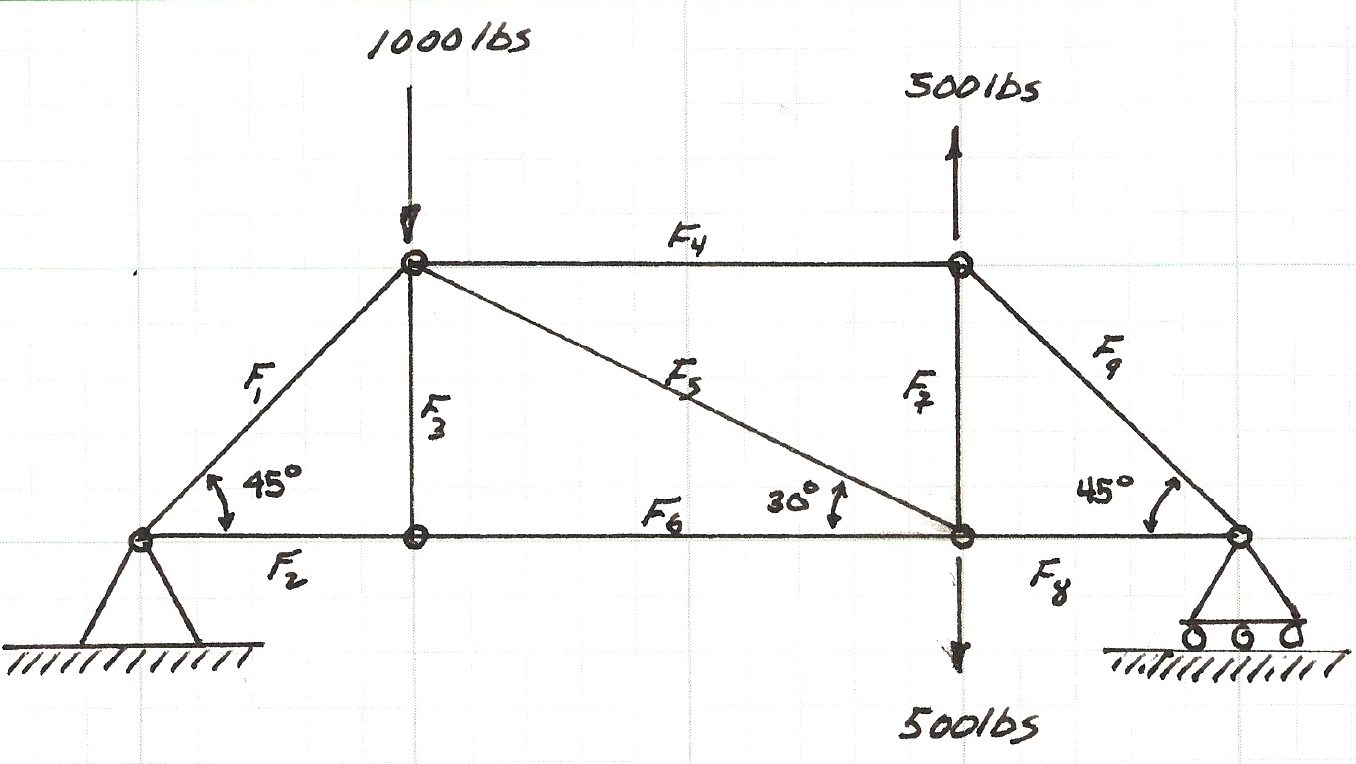
This notebook will illustrate how to leverage a linear systems solver(s) to analyze the truss. The approach uses concepts from statics and computational thinking.
From statics
method of joints (for reactions and internal forcez)
direction cosines
From computational thinking
read input file
construct linear system \(\textbf{Ax=b}\); solve for \(\textbf{x}\)
report results
Before even contemplating writing/using a program we need to build a mathematical model of the truss and assemble the system of linear equations that result from the model.
So the first step is to sketch a free-body-diagram as below and build a node naming convention and force names.
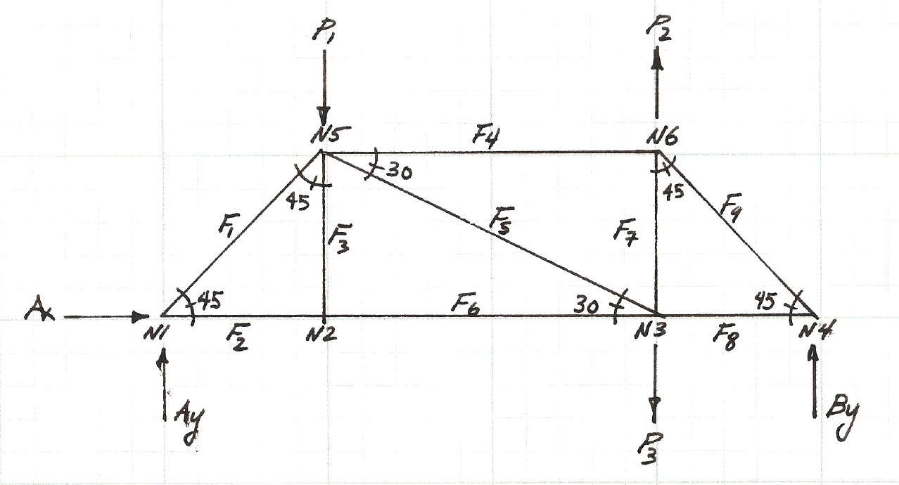
Next we will write the force balance for each of the six nodes (\(N1\)-\(N6\)), which will produce a total of 12 equations in the 12 unknowns (the 9 member forces, and 3 reactions).
The figure below is the force balance for node \(N1\), the two force equations (for the horizontal, \(x\), direction and the vertical, \(y\), direction) are listed below the figure.
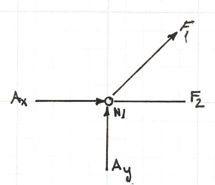
The equation above is the force balance equation pair for the node. The \(x\) component equation will later be named \(N1_x\) to indicate it arises from Node 1, \(x\) component equation. A similar notation convention will also be adopted for the \(y\) component equation. There will be an equation pair for each node.
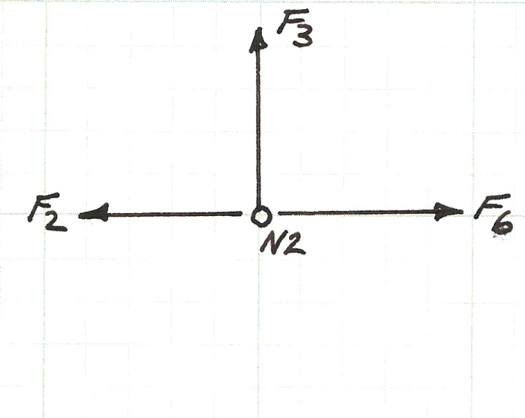
Below is a sketch of the force balance for node \(N2\), the two force equations (for the horizontal, \(x\), direction and the vertical, \(y\), direction) are listed below the figure.
Below is a sketch of the force balance for node \(N3\), the two force equations (for the horizontal, \(x\), direction and the vertical, \(y\), direction) are listed below the figure.
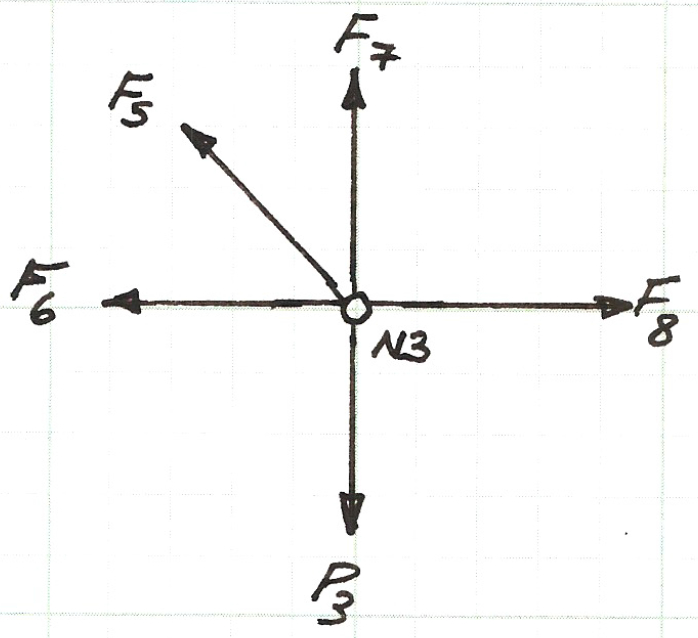
Above is the force balance equation pair for node \(N3\).
Below is a sketch of the force balance for node \(N4\), the two force equations (for the horizontal, \(x\), direction and the vertical, \(y\), direction) are listed below the figure.
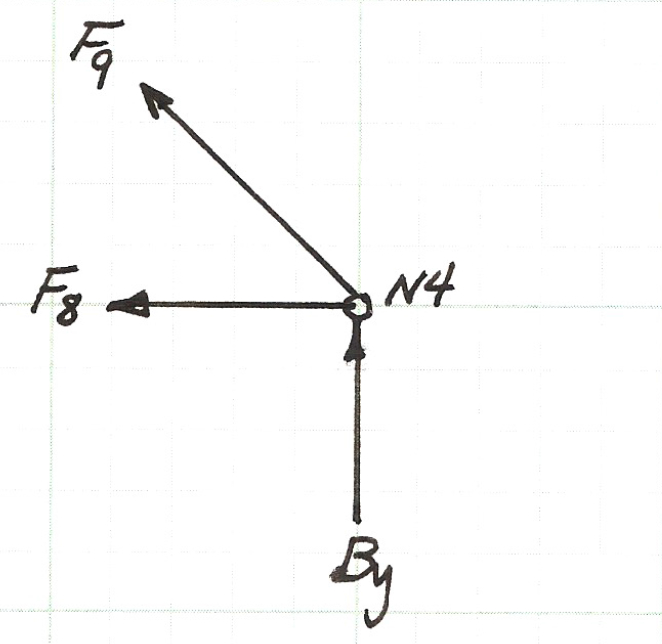
Above is the force balance equation pair for node \(N4\).
Below is a sketch of the force balance for node \(N5\), the two force equations (for the horizontal, \(x\), direction and the vertical, \(y\), direction) are listed below the figure.
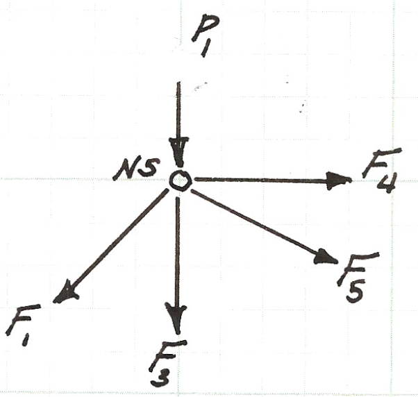
Above is the force balance equation pair for node \(N5\).
Below is a sketch of the force balance for node \(N6\), the two force equations (for the horizontal, \(x\), direction and the vertical, \(y\), direction) are listed below the figure.
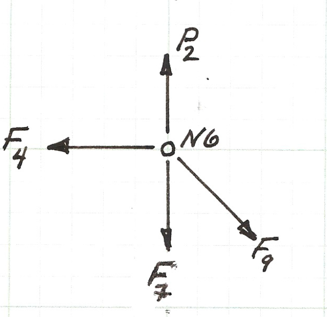
Above is the force balance equation pair for node \(N6\).
The next step is to gather the equation pairs into a system of linear equations.
We will move the known loads to the right hand side and essentially construct the matrix equation \(\mathbf{A}\mathbf{x} = \mathbf{b}\).
The system below is a matrix representation of the equation pairs with the forces moved to the right hand side \(\mathbf{b} = RHS\).
In the system, the rows are labeled on the left-most column with their node-related equation name.
Thus each row of the matrix corresponds to an equation derived from a node.
The columns are labeled with their respective unknown force (except the last column, which represents the right-hand-side of the system of linear equations).
Thus the coefficient in each column corresponds to a force in each node equation.
The sign of the coefficient refers to the assumed direction the force acts.
In the analysis all the members were assumed to be in tension (except for the reaction forces).
If a coefficient has a value of zero in a particular row, then that force does no act at the node to which the row corresponds.
From this representation the transition to the formal vector-matrix representation is straightforward.
The various matrices above are entere into text files named A.txt and B.txt
# list contents of the A matrix, uses call to OS host
#!(type A.txt) # windoze method
!(cat A.txt) # linux, macOS
0.707106781	1	0	0	0	0	0	0	0	1	0	0

0.707106781	0	0	0	0	0	0	0	0	0	1	0

0	-1	0	0	0	1	0	0	0	0	0	0

0	0	1	0	0	0	0	0	0	0	0	0

0	0	0	0	-0.866	-1	0	1	0	0	0	0

0	0	0	0	0.5	0	1	0	0	0	0	0

0	0	0	0	0	0	0	-1	-0.707106781	0	0	0

0	0	0	0	0	0	0	0	0.707106781	0	0	1

-0.707106781	0	0	1	0.866	0	0	0	0	0	0	0

-0.707106781	0	-1	0	-0.5	0	0	0	0	0	0	0

0	0	0	-1	0	0	0	0	0.707106781	0	0	0

0	0	0	0	0	0	-1	0	-0.707106781	0	0	0
# list contents of RHS or b vector
#!(type B.txt) # winders method
!(cat B.txt) # linux, macOS
0.0

0.0

0.0

0.0

0.0

500.0

0.0

0.0

0.0

1000.0

0.0

-500.0
Now we use our solver tools, here I have not done much on tidy output, thats left for the reader.
# LinearSolverPivot.py
# linearsolver with pivoting adapted from
# https://stackoverflow.com/questions/31957096/gaussian-elimination-with-pivoting-in-python/31959226

def linearsolver(A,b):
    n = len(A)
    M = A # this is equivalence, A is destroyed by algorithm

    i = 0
    for x in M:
     x.append(b[i])
     i += 1

    for k in range(n):
     for i in range(k,n):
       if abs(M[i][k]) > abs(M[k][k]):
          M[k], M[i] = M[i],M[k]
       else:
          pass

     for j in range(k+1,n):
         q = float(M[j][k]) / M[k][k]
         for m in range(k, n+1):
            M[j][m] -=  q * M[k][m]

    x = [0 for i in range(n)]

    x[n-1] =float(M[n-1][n])/M[n-1][n-1]
    for i in range (n-1,-1,-1):
      z = 0
      for j in range(i+1,n):
          z = z  + float(M[i][j])*x[j]
      x[i] = float(M[i][n] - z)/M[i][i]
#    print (x)
    return(x)

amatrix = [] # null list to store matrix reads
bvector = []
rowNumA = 0
colNumA = 0
rowNumB = 0
afile = open("A.txt","r")  # connect and read file for MATRIX A
for line in afile:
    amatrix.append([float(n) for n in line.strip().split()])
    rowNumA += 1
afile.close() # Disconnect the file
colNumA = len(amatrix[0])
afile = open("B.txt","r")  # connect and read file for MATRIX B
for line in afile:
    bvector.append(float(line))  # vector read different -- just float the line
    rowNumB += 1
afile.close() # Disconnect the file
#print (bvector)
if rowNumA != rowNumB:   # check the arrays
    print ("row ranks not same -- aborting now")
    quit()
else:
    print ("row ranks same -- continuing operation")
# print all columns each row
cmatrix = [[0 for j in range(colNumA)]for i in range(rowNumA)]
dmatrix = [[0 for j in range(colNumA)]for i in range(rowNumA)]
xvector = [0 for i in range(rowNumA)]
dvector = [0 for i in range(rowNumA)]
for i in range(0,rowNumA,1):
    print (amatrix[i][0:colNumA], bvector[i])
print ("-----------------------------")
# copy amatrix into cmatrix
cmatrix = [[amatrix[i][j] for j in range(colNumA)]for i in range(rowNumA)]
dmatrix = [[amatrix[i][j] for j in range(colNumA)]for i in range(rowNumA)]
dvector = [bvector[i] for i in range(rowNumA)]
xvector = linearsolver(cmatrix,bvector) # send cmatrix the copy of amatrix; the solver destroys the inputs, hence the copies
for i in range(0,rowNumA,1):
    print (xvector[i])
print ("-----------------------------")
row ranks same -- continuing operation
[0.707106781, 1.0, 0.0, 0.0, 0.0, 0.0, 0.0, 0.0, 0.0, 1.0, 0.0, 0.0] 0.0
[0.707106781, 0.0, 0.0, 0.0, 0.0, 0.0, 0.0, 0.0, 0.0, 0.0, 1.0, 0.0] 0.0
[0.0, -1.0, 0.0, 0.0, 0.0, 1.0, 0.0, 0.0, 0.0, 0.0, 0.0, 0.0] 0.0
[0.0, 0.0, 1.0, 0.0, 0.0, 0.0, 0.0, 0.0, 0.0, 0.0, 0.0, 0.0] 0.0
[0.0, 0.0, 0.0, 0.0, -0.866, -1.0, 0.0, 1.0, 0.0, 0.0, 0.0, 0.0] 0.0
[0.0, 0.0, 0.0, 0.0, 0.5, 0.0, 1.0, 0.0, 0.0, 0.0, 0.0, 0.0] 500.0
[0.0, 0.0, 0.0, 0.0, 0.0, 0.0, 0.0, -1.0, -0.707106781, 0.0, 0.0, 0.0] 0.0
[0.0, 0.0, 0.0, 0.0, 0.0, 0.0, 0.0, 0.0, 0.707106781, 0.0, 0.0, 1.0] 0.0
[-0.707106781, 0.0, 0.0, 1.0, 0.866, 0.0, 0.0, 0.0, 0.0, 0.0, 0.0, 0.0] 0.0
[-0.707106781, 0.0, -1.0, 0.0, -0.5, 0.0, 0.0, 0.0, 0.0, 0.0, 0.0, 0.0] 1000.0
[0.0, 0.0, 0.0, -1.0, 0.0, 0.0, 0.0, 0.0, 0.707106781, 0.0, 0.0, 0.0] 0.0
[0.0, 0.0, 0.0, 0.0, 0.0, 0.0, -1.0, 0.0, -0.707106781, 0.0, 0.0, 0.0] -500.0
-----------------------------
-1035.2710218174145
732.0471596998927
0.0
-267.9528403001072
-535.9056806002143
732.0471596998927
767.9528403001071
267.95284030010714
-378.94254092877543
0.0
732.0471596998927
267.9528403001072
-----------------------------
Now lets do the same tasks using numpy
import numpy
# already read in the arrays
A = numpy.array(amatrix)
Ainv = numpy.linalg.inv(A)
b = numpy.array(bvector)
x = Ainv@b
for i in range(0,len(x)):
    print(x[i])
-1035.2710218174143
732.0471596998927
0.0
-267.95284030010714
-535.9056806002143
732.0471596998927
767.9528403001071
267.9528403001071
-378.9425409287754
-3.9202487786118276e-14
732.0471596998927
267.95284030010714
import numpy
# need to read in the arrays
A = numpy.loadtxt("A.txt")
b = numpy.loadtxt("B.txt")
Ainv = numpy.linalg.inv(A)
x = Ainv@b
for i in range(0,len(x)):
    print(x[i])
-1035.2710218174143
732.0471596998927
0.0
-267.95284030010714
-535.9056806002143
732.0471596998927
767.9528403001071
267.9528403001071
-378.9425409287754
-3.9202487786118276e-14
732.0471596998927
267.95284030010714
import numpy
# need to read in the arrays
A = numpy.loadtxt("A.txt")
b = numpy.loadtxt("B.txt")
x = numpy.linalg.solve(A,b) # avoid inversion and just solve the linear system
for i in range(0,len(x)):
    print(x[i])
-1035.2710218174145
732.0471596998927
0.0
-267.9528403001072
-535.9056806002143
732.0471596998927
767.9528403001071
267.95284030010714
-378.94254092877543
-3.9202487786118276e-14
732.0471596998927
267.95284030010714
References
Johnson, J. (2020). Python Numpy Tutorial (with Jupyter and Colab). Retrieved September 15, 2020, from https://cs231n.github.io/python-numpy-tutorial/
Willems, K. (2019). (Tutorial) Python NUMPY Array TUTORIAL. Retrieved September 15, 2020, from https://www.datacamp.com/community/tutorials/python-numpy-tutorial?utm_source=adwords_ppc
Willems, K. (2017). NumPy Cheat Sheet: Data Analysis in Python. Retrieved September 15, 2020, from https://www.datacamp.com/community/blog/python-numpy-cheat-sheet
W3resource. (2020). NumPy: Compare two given arrays. Retrieved September 15, 2020, from https://www.w3resource.com/python-exercises/numpy/python-numpy-exercise-28.php
Sorting https://www.programiz.com/python-programming/methods/list/sort
Overland, B. (2018). Python Without Fear. Addison-Wesley ISBN 978-0-13-468747-6.
Grus, Joel (2015). Data Science from Scratch: First Principles with Python O’Reilly Media. Kindle Edition.
Precord, C. (2010) wxPython 2.8 Application Development Cookbook Packt Publishing Ltd. Birmingham , B27 6PA, UK ISBN 978-1-849511-78-0.
Laboratory 9
Examine (click) Laboratory 9 as a webpage at Laboratory 9.html
Download (right-click, save target as …) Laboratory 9 as a jupyterlab notebook from Laboratory 9.ipynb
Exercise Set 9
Examine (click) Exercise Set 9 as a webpage at Exercise 9.html
Download (right-click, save target as …) Exercise Set 9 as a jupyterlab notebook at Exercise Set 9.ipynb