ENGR 1330 Computational Thinking with Data Science
Copyright © 2021 Theodore G. Cleveland and Farhang Forghanparast
Last GitHub Commit Date: 13 July 2021
5: Algorithm Building Blocks
Three building blocks (structures): sequence, selection , repetition (loops)
Sequence
Selection
Repetition
Structured FOR loops
Structured WHILE loops
Representing computational processes with flowcharts, a graphical abstraction
Objectives
Develop awareness of fundamental structures in algorithms:
sequence
selection
repetition
Develop awareness of loops, and their utility in automation.
To understand loop types available in Python.
To understand and implement loops in various examples and configurations.
Develop awareness of flowcharts as a tool for:
Post-development documentation
Pre-development program design
Algorithm Structures
The three fundamental structures are sequence, selection, and repetition.
Sequence
Sequential processing are steps performed in sequence, one after another. A default spreadsheet computation from top-to-bottom is a sequential process.
Reliability Example Suppose we wish to estimate the reliability of a system comprised of many indetical parts iused in multiple places in a design, for instance rivets on an airplane wing. Using a Bernoulli model (which you will see in your statistics class) we can estimate the collective reliability of the system (all the parts work as desired). The reliability is expressed as the fraction of time that no parts have failed, if the fraction is small we would want to either improve part reliability, or ensure redundancy so the system can function with broken parts.
Let \(p\) be the probability a single component is good and \(N\) be the total number of components in the system that work together in a “series” context. The reliability, or the percentage of time that none of the components have failed is given by the Bernoulli equation:
Suppose we want a script to read in a component probability and count, and estimate system reliability – we can apply our problem solving protocol and JupyterLab to do so, and the task will be mostly sequential
Step 1 Problem Statement Estimate the reliability of a component in an instrument relative to a group of components using a Bernoulli approximation.
Step 2 Input/Output Decomposition Inputs are the reliability of a single component and the number of components working together in a system, output is estimate of system reliability, governing principle is the Bernoulli equation above.
Step 3 By-Hand Example Suppose the system is a small FPGA with 20 transistors, each with reliability of 96-percent. The entire array reliability is
Step 4 Algorithm Development Decompose the computation problem as:
Read reliability of a single component
Read how many components
Compute reliability by bernoulli model
Report result
Step 5 Scripting Written as a sequence we can have
component = float(input('Component Reliability (percentage-numeric)?'))
howmany = int(input('Number of Components (integer-numeric)?'))
reliability = 100.0*(component/100.0)**howmany
print('Component Reliability: ',round(component,1))
print('Number of Components : ',howmany)
print('System Reliability is : ',round(reliability,1),'%')
Step 6 Refinement We have tested the script with the by-hand example, no refinement really needed here, but lets apply to new conditions
component = float(input('Component Reliability (percentage-numeric)?'))
howmany = int(input('Number of Components (integer-numeric)?'))
reliability = 100.0*(component/100.0)**howmany
print('Component Reliability: ',round(component,1))
print('Number of Components : ',howmany)
print('System Reliability is : ',round(reliability,1),'%')
Selection Structures
Selection via conditional statements is an important step in algorithm design; its one way to control the flow of execution of a program.
Conditional statements in Python include:
ifstatement is true, then do …if....elsestatement is true, then do …, otherwise do something elseif....elif....elsestatement is true, then do …, if something else is true then do …, otherwise do …
Conditional statements are logical expressions that evaluate as TRUE or FALSE and using these results to perform further operations based on these conditions. All flow control in a program depends on evaluating conditions. The program will proceed diferently based on the outcome of one or more conditions - really sophisticated AI programs are a collection of conditions and correlations.
Expressed in a flowchart a block if statement looks like:
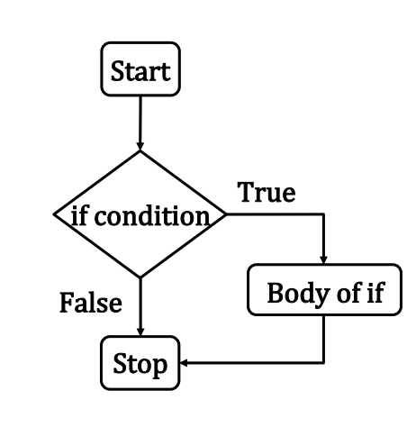
As psuedo code:
if(condition is true):
    do stuff
Amazon knowing what you kind of want is based on correlations of your past behavior compared to other peoples similar, but more recent behavior, and then it uses conditional statements to decide what item to offer you in your recommendation items. It’s spooky, but ultimately just a program running in the background trying to make your money theirs.
Comparison
The most common conditional operation is comparison. If we wish to compare whether two variables are the same we use the == (double equal sign).
For example x == y means the program will ask whether x and y have the same value. If they do, the result is TRUE if not then the result is FALSE.
Other comparison signs are != does NOT equal, < smaller than, > larger than, <= less than or equal, and >= greater than or equal.
There are also three logical operators when we want to build multiple compares
(multiple conditioning); these are and, or, and not.
The and operator returns TRUE if (and only if) all conditions are TRUE.
For instance 5 == 5 and 5 < 6 will return a TRUE because both conditions are true.
The or operator returns TRUE if at least one condition is true.
If all conditions are FALSE, then it will return a FALSE. For instance 4 > 3 or 17 > 20 or 3 == 2 will return TRUEbecause the first condition is true.
The not operator returns TRUE if the condition after the not keyword is false. Think of it
as a way to do a logic reversal.
Block if statement
The if statement is a common flow control statement.
It allows the program to evaluate if a certain condition is satisfied and to perform a designed action based on the result of the evaluation. The structure of an if statement is
if condition1 is met:
    do A
elif condition 2 is met:
    do b
elif condition 3 is met:
    do c
else:
    do e
The elif means “else if”. The : colon is an important part of the structure it tells where the action begins. Also there are no scope delimiters like (), or {} .
Instead Python uses indentation to isolate blocks of code.
This convention is hugely important - many other coding environments use delimiters (called scoping delimiters), but Python does not. The indentation itself is the scoping delimiter.
Inline if statement
An inline if statement is a simpler form of an if statement and is more convenient if you
only need to perform a simple conditional task.
The syntax is:
do TaskA `if` condition is true `else` do TaskB
An example would be
myInt = 3
num1 = 12 if myInt == 0 else 13
num1
An alternative way is to enclose the condition in brackets for some clarity like
myInt = 3
num1 = 12 if (myInt == 0) else 13
num1
In either case the result is that num1 will have the value 13 (unless you set myInt to 0).
One can also use if to construct extremely inefficient loops.
Repetition and Loops
Computational thinking (CT) concepts involved are:
Decomposition: Break a problem down into smaller pieces; the body of tasks in one repetition of a loop represent decomposition of the entire sets of repeated activitiesPattern Recognition: Finding similarities between things; the body of tasks in one repetition of a loop is the pattern, the indices and components that change are how we leverage reuseAbstraction: Pulling out specific differences to make one solution work for multiple problemsAlgorithms: A list of steps that you can follow to finish a task
The action of doing something over and over again (repetition) is called a loop. Basically, Loops repeats a portion of code a finite number of times until a process is complete. Repetitive tasks are very common and essential in programming. They save time in coding, minimize coding errors, and leverage the speed of electronic computation.
Loop Analogs
If you think any mass manufacturing process, we apply the same process again and again. Even for something very simple such as preparing a peanut butter sandwich:
Consider the flowchart in Figure 1, it represents a decomposition of sandwich assembly, but at a high level – for instance, Gather Ingredients contains a lot of substeps that would need to be decomposed if fully automated assembly were to be accomplished; nevertheless lets stipulate that this flowchart will indeed construct a single sandwich.
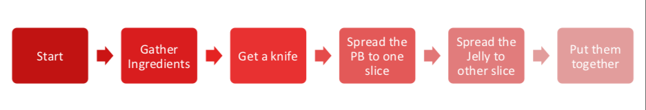
If we need to make 1000 peanut butter sandwichs we would then issue a directive to:
Implement sandwich assembly, repeat 999 times (repeat is the loop structure) (A serial structure, 1 sandwich artist, doing same job over and over again)
OR
Implement 1000 sandwich assembly threads (A parallel structure, 1000 sandwich artists doing same job once)
In general because we dont want to idle 999 sandwich artists, we would choose the serial structure, which frees 999 people to ask the existential question “would you like fries with that?”
All cynicism aside, an automated process such as a loop, is typical in computational processing.
Note
NVIDIA CUDA, and AMD OpenGL compilers can detect the structure above, and if there are enough GPU threads available , create the 1000 sandwich artists (1000 GPU threads), and run the process in parallel – the actual workload is unchanged in a thermodynamic sense, but the apparent time (in human terms) spent in sandwich creation is a fraction of the serial approach. This kind of parallelization is called “unrolling the loop”, and is a pretty common optimization step during compilation. This kind of programming is outside the scope of this class.
Main attractiveness of loops is:
Leveraging
pattern matchingandautomationCode is more organized and shorter,because a loop is a sequence of instructions that is continually repeated until a certain condition is reached.
There are 2 main types loops based on the repetition control condition; for loops and whileloops.
For Loop (Count controlled repetition structure)
Count-controlled repetition is also called definite repetition because the number of repetitions is known before the loop begins executing. When we do not know in advance the number of times we want to execute a statement, we cannot use count-controlled repetition. In such an instance, we would use sentinel-controlled repetition.
A count-controlled repetition will exit after running a certain number of times. The count is kept in a variable called an index or counter. When the index reaches a certain value (the loop bound) the loop will end.
Count-controlled repetition requires
control variable (or loop counter)
initial value of the control variable
increment (or decrement) by which the control variable is modified each iteration through the loop
condition that tests for the final value of the control variable
We can use both for and while loops, for count controlled repetition, but the for loop in combination with the range() function is more common.
Structured FOR loop
We have seen the for loop already, but we will formally introduce it here. The for loop executes a block of code repeatedly until the condition in the for statement is no longer true.
Looping through an iterable
An iterable is anything that can be looped over - typically a list, string, or tuple. The syntax for looping through an iterable is illustrated by an example.
First a generic syntax
for a in iterable:
print(a)
Notice our friends the colon : and the indentation.
The range() function to create an iterable
The range(begin,end,increment) function will create an iterable starting at a value of begin, in steps defined by increment (begin += increment), ending at end.
So a generic syntax becomes
for a in range(begin,end,increment):
print(a)
The examples that follow are count-controlled repetition (increment skip if greater)
Example for loops
# sum numbers from 1 to n
howmany = int(input('Enter N'))
accumulator = 0.0
for i in range(0,howmany+1,1):
    accumulator = accumulator + float(i)
    print(i)
print( 'Sum from 1 to ',howmany, 'is %.3f' % accumulator  )
# sum even numbers from 1 to n
howmany = int(input('Enter N'))
accumulator = 0.0
for i in range(1,howmany+1,1):
    if i%2 == 0:
        print(i)
        accumulator = accumulator + float(i)
print( 'Sum of Evens from 1 to ',howmany, 'is %.3f' % accumulator  )
howmany = int(input('Enter N'))
linetoprint=''
for i in range(1,howmany+1,1):
    linetoprint=linetoprint + '?'
    print(linetoprint)
Sentinel-controlled repetition.
When loop control is based on the value of what we are processing, sentinel-controlled repetition is used. Sentinel-controlled repetition is also called indefinite repetition because it is not known in advance how many times the loop will be executed. It is a repetition procedure for solving a problem by using a sentinel value (also called a signal value, a dummy value or a flag value) to indicate “end of process”. The sentinel value itself need not be a part of the processed data.
One common example of using sentinel-controlled repetition is when we are processing data from a file and we do not know in advance when we would reach the end of the file.
We can use both for and while loops, for Sentinel controlled repetition, but the while loop is more common.
Structured WHILE loop
The while loop repeats a block of instructions inside the loop while a condition remainsvtrue.
First a generic syntax
while condition is true:
    execute a
    execute b
....
Notice our friends the colon : and the indentation again.
Example while loops
# sum numbers from 1 to n
howmany = int(input('Enter N'))
accumulator = 0.0
counter = 1
while counter <= howmany:
    accumulator = accumulator + float(counter)
    counter += 1
print( 'Sum from 1 to ',howmany, 'is %.3f' % accumulator  )
# sum even numbers from 1 to n
howmany = int(input('Enter N'))
accumulator = 0.0
counter = 1
while counter <= howmany:
    if counter%2 == 0:
        accumulator = accumulator + float(counter)
    counter += 1
print( 'Sum of Evens 1 to ',howmany, 'is %.3f' % accumulator  )
howmany = int(input('Enter N'))
linetoprint=''
counter = 1
while counter <= howmany:
    linetoprint=linetoprint + '?'
    counter += 1
    print(linetoprint)
Nested Repetition
Nested repetition is when a control structure is placed inside of the body or main part of another control structure.
break to exit out of a loop
Sometimes you may want to exit the loop when a certain condition different from the counting condition is met. Perhaps you are looping through a list and want to exit when you find the first element in the list that matches some criterion. The break keyword is useful for such an operation.
For example run the following program:
#
j = 0
for i in range(0,9,1):
    j += 2
    print ("i = ",i,"j = ",j)
    if j == 14:
        break
i =  0 j =  2
i =  1 j =  4
i =  2 j =  6
i =  3 j =  8
i =  4 j =  10
i =  5 j =  12
i =  6 j =  14
j = 0
for i in range(0,5,1):
    j += 2
    print( "i = ",i,"j = ",j)
    if j == 7:
        break
i =  0 j =  2
i =  1 j =  4
i =  2 j =  6
i =  3 j =  8
i =  4 j =  10
In the first case, the for loop only executes 3 times before the condition j == 6 is TRUE and the loop is exited. In the second case, j == 7 never happens so the loop completes all its anticipated traverses.
In both cases an if statement was used within a for loop. Such “mixed” control structures
are quite common (and pretty necessary).
A while loop contained within a for loop, with several if statements would be very common and such a structure is called nested control.
There is typically an upper limit to nesting but the limit is pretty large - easily in the
hundreds. It depends on the language and the system architecture ; suffice to say it is not
a practical limit except possibly for general-domain AI applications.
We can also do mundane activities and leverage loops, arithmetic, and format codes to make useful tables like
import math # package that contains cosine
print("     Cosines     ")
print("   x   ","|"," cos(x) ")
print("--------|--------")
for i in range(0,157,1):
    x = float(i)*0.1
    print("%.3f" % x, "  |", " %.4f "  % math.cos(x)) # note the format code and the placeholder % and syntax
     Cosines
   x    |  cos(x)
--------|--------
0.000   |  1.0000
0.100   |  0.9950
0.200   |  0.9801
0.300   |  0.9553
0.400   |  0.9211
0.500   |  0.8776
0.600   |  0.8253
0.700   |  0.7648
0.800   |  0.6967
0.900   |  0.6216
1.000   |  0.5403
1.100   |  0.4536
1.200   |  0.3624
1.300   |  0.2675
1.400   |  0.1700
1.500   |  0.0707
1.600   |  -0.0292
1.700   |  -0.1288
1.800   |  -0.2272
1.900   |  -0.3233
2.000   |  -0.4161
2.100   |  -0.5048
2.200   |  -0.5885
2.300   |  -0.6663
2.400   |  -0.7374
2.500   |  -0.8011
2.600   |  -0.8569
2.700   |  -0.9041
2.800   |  -0.9422
2.900   |  -0.9710
3.000   |  -0.9900
3.100   |  -0.9991
3.200   |  -0.9983
3.300   |  -0.9875
3.400   |  -0.9668
3.500   |  -0.9365
3.600   |  -0.8968
3.700   |  -0.8481
3.800   |  -0.7910
3.900   |  -0.7259
4.000   |  -0.6536
4.100   |  -0.5748
4.200   |  -0.4903
4.300   |  -0.4008
4.400   |  -0.3073
4.500   |  -0.2108
4.600   |  -0.1122
4.700   |  -0.0124
4.800   |  0.0875
4.900   |  0.1865
5.000   |  0.2837
5.100   |  0.3780
5.200   |  0.4685
5.300   |  0.5544
5.400   |  0.6347
5.500   |  0.7087
5.600   |  0.7756
5.700   |  0.8347
5.800   |  0.8855
5.900   |  0.9275
6.000   |  0.9602
6.100   |  0.9833
6.200   |  0.9965
6.300   |  0.9999
6.400   |  0.9932
6.500   |  0.9766
6.600   |  0.9502
6.700   |  0.9144
6.800   |  0.8694
6.900   |  0.8157
7.000   |  0.7539
7.100   |  0.6845
7.200   |  0.6084
7.300   |  0.5261
7.400   |  0.4385
7.500   |  0.3466
7.600   |  0.2513
7.700   |  0.1534
7.800   |  0.0540
7.900   |  -0.0460
8.000   |  -0.1455
8.100   |  -0.2435
8.200   |  -0.3392
8.300   |  -0.4314
8.400   |  -0.5193
8.500   |  -0.6020
8.600   |  -0.6787
8.700   |  -0.7486
8.800   |  -0.8111
8.900   |  -0.8654
9.000   |  -0.9111
9.100   |  -0.9477
9.200   |  -0.9748
9.300   |  -0.9922
9.400   |  -0.9997
9.500   |  -0.9972
9.600   |  -0.9847
9.700   |  -0.9624
9.800   |  -0.9304
9.900   |  -0.8892
10.000   |  -0.8391
10.100   |  -0.7806
10.200   |  -0.7143
10.300   |  -0.6408
10.400   |  -0.5610
10.500   |  -0.4755
10.600   |  -0.3853
10.700   |  -0.2913
10.800   |  -0.1943
10.900   |  -0.0954
11.000   |  0.0044
11.100   |  0.1042
11.200   |  0.2030
11.300   |  0.2997
11.400   |  0.3935
11.500   |  0.4833
11.600   |  0.5683
11.700   |  0.6476
11.800   |  0.7204
11.900   |  0.7861
12.000   |  0.8439
12.100   |  0.8932
12.200   |  0.9336
12.300   |  0.9647
12.400   |  0.9862
12.500   |  0.9978
12.600   |  0.9994
12.700   |  0.9911
12.800   |  0.9728
12.900   |  0.9449
13.000   |  0.9074
13.100   |  0.8610
13.200   |  0.8059
13.300   |  0.7427
13.400   |  0.6722
13.500   |  0.5949
13.600   |  0.5117
13.700   |  0.4234
13.800   |  0.3308
13.900   |  0.2349
14.000   |  0.1367
14.100   |  0.0372
14.200   |  -0.0628
14.300   |  -0.1621
14.400   |  -0.2598
14.500   |  -0.3549
14.600   |  -0.4465
14.700   |  -0.5336
14.800   |  -0.6154
14.900   |  -0.6910
15.000   |  -0.7597
15.100   |  -0.8208
15.200   |  -0.8737
15.300   |  -0.9179
15.400   |  -0.9530
15.500   |  -0.9785
15.600   |  -0.9942
The continue statement
The continue instruction skips the block of code after it is executed for that iteration. It is best illustrated by an example.
j = 0
for i in range(0,5,1):
    j += 2
    print ("\n i = ", i , ", j = ", j) #here the \n is a newline command
    if j == 6:
        continue
    print(" this message will be skipped over if j = 6 ") # still within the loop, so the skip is implemented
 i =  0 , j =  2
 this message will be skipped over if j = 6

 i =  1 , j =  4
 this message will be skipped over if j = 6

 i =  2 , j =  6

 i =  3 , j =  8
 this message will be skipped over if j = 6

 i =  4 , j =  10
 this message will be skipped over if j = 6
The try, except structure
An important control structure (and a pretty cool one for error trapping) is the try, except
statement.
The statement controls how the program proceeds when an error occurs in an instruction. The structure is really useful to trap likely errors (divide by zero, wrong kind of input) yet let the program keep running or at least issue a meaningful message to the user.
The syntax is:
try:
do something
except:
do something else if ``do something'' returns an error
Here is a really simple, but hugely important example:
#MyErrorTrap.py
x = 12.
y = 12.
while y >= -12.: # sentinel controlled repetition
    try:
        print ("x = ", x, "y = ", y, "x/y = ", x/y)
    except:
        print ("error divide by zero")
    y -= 1
x =  12.0 y =  12.0 x/y =  1.0
x =  12.0 y =  11.0 x/y =  1.0909090909090908
x =  12.0 y =  10.0 x/y =  1.2
x =  12.0 y =  9.0 x/y =  1.3333333333333333
x =  12.0 y =  8.0 x/y =  1.5
x =  12.0 y =  7.0 x/y =  1.7142857142857142
x =  12.0 y =  6.0 x/y =  2.0
x =  12.0 y =  5.0 x/y =  2.4
x =  12.0 y =  4.0 x/y =  3.0
x =  12.0 y =  3.0 x/y =  4.0
x =  12.0 y =  2.0 x/y =  6.0
x =  12.0 y =  1.0 x/y =  12.0
error divide by zero
x =  12.0 y =  -1.0 x/y =  -12.0
x =  12.0 y =  -2.0 x/y =  -6.0
x =  12.0 y =  -3.0 x/y =  -4.0
x =  12.0 y =  -4.0 x/y =  -3.0
x =  12.0 y =  -5.0 x/y =  -2.4
x =  12.0 y =  -6.0 x/y =  -2.0
x =  12.0 y =  -7.0 x/y =  -1.7142857142857142
x =  12.0 y =  -8.0 x/y =  -1.5
x =  12.0 y =  -9.0 x/y =  -1.3333333333333333
x =  12.0 y =  -10.0 x/y =  -1.2
x =  12.0 y =  -11.0 x/y =  -1.0909090909090908
x =  12.0 y =  -12.0 x/y =  -1.0
So this silly code starts with x fixed at a value of 12, and y starting at 12 and decreasing by 1 until y equals -1. The code returns the ratio of x to y and at one point y is equal to zero and the division would be undefined. By trapping the error the code can issue us a measure and keep running.
Modify the script as shown below,Run, and see what happens
#NoErrorTrap.py
x = 12.
y = 12.
while y >= -12.: # sentinel controlled repetition
    print ("x = ", x, "y = ", y, "x/y = ", x/y)
    y -= 1
Flowcharts
What is a Flowchart?
A flowchart is a type of diagram that represents a workflow or process. A flowchart can also be defined as a diagrammatic representation of an algorithm, a step-by-step approach to solving a task.

The flowchart shows the steps as boxes of various kinds, and their order by connecting the boxes with arrows. This diagrammatic representation illustrates a solution model to a given problem. Flowcharts are used in analyzing, designing, documenting or managing a process or program in various fields.
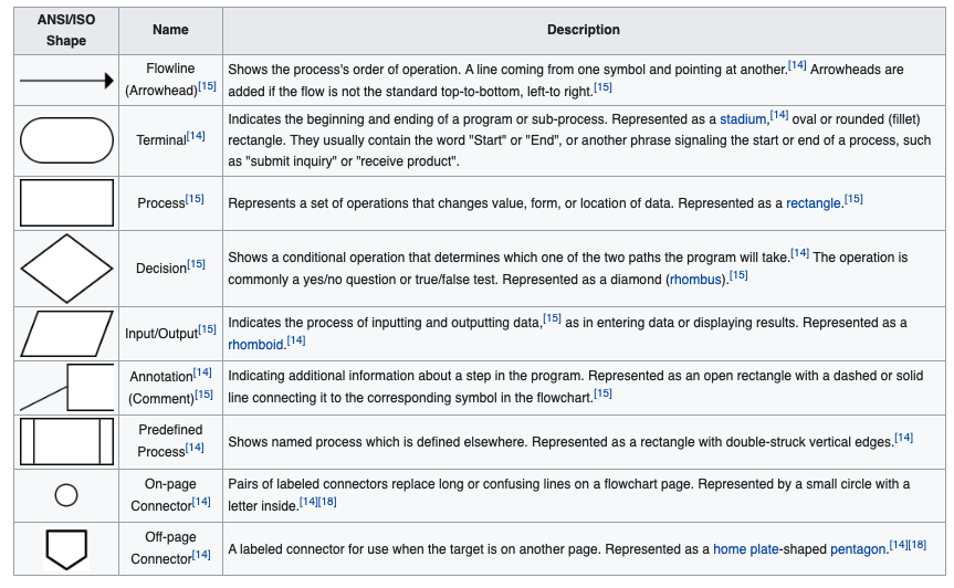
There is a symbol convention (a language) as depicted in Figure 2 below (from: https://en.wikipedia.org/wiki/Flowchart)
IBM engineers implemented programming flowcharts based upon Goldstine and von Neumann’s unpublished report, “Planning and coding of problems for an electronic computing instrument, Part II, Volume 1” (1947), which is reproduced in von Neumann’s collected works.
The flowchart became a popular tool for describing computer algorithms, but its popularity decreased in the 1970s, when interactive computer terminals and third-generation programming languages became common tools for computer programming, since algorithms can be expressed more concisely as source code in such languages. Often pseudo-code is used, which uses the common idioms of such languages without strictly adhering to the details of a particular one.
Nowadays flowcharts are still used for describing computer algorithms.[9] Modern techniques such as UML activity diagrams and Drakon-charts can be considered to be extensions of the flowchart.
Nearly all flowcharts focus on on some kind of control, rather than on the particular flow itself! While quaint today, they are an effective way to document processes in a program and visualize structures. We recomend you get in the habit of making rudimentary flowcharts, at least at the supervisory level (the sandwich chart above)
How are they useful?
(paraphrased from https://www.breezetree.com/articles/top-reasons-to-flowchart)
Sometimes it’s more effective to visualize something graphically that it is to describe it with words. That is the essence of what flowcharts do for you. Flowcharts explain a process clearly through symbols and text. Moreover, flowcharts give you the gist of the process flow in a single glance. The following are some of the more salient reasons to use flowcharts.
Process Documentation / Training Materials Another common use for flowcharts is to create process documentation. Although this reason overlaps with regulatory and quality management requirements (below), many non-regulated businesses use flowcharts for their documentation as well. These can range in form from high-level procedures to low-level, detailed work instructions.
You may think that this applies mainly to large organizations, but small companies can greatly benefit from flowcharting their processes as well. Small enterprises need to be nimble and organized. Standardizing their processes is a great way to achieve this. In fact, the popular entrepreneurial book The E-Myth Revisited: Why Most Small Businesses Don’t Work and What to Do About It by Michael Gerber is based on the fact that small businesses are more likely to succeed if they treat their operations like a franchise. in a nutshell, this means standardizing and documenting their business processes. There’s no better way to do that than with flowcharts, right?
Training materials are often created using flowcharts because they’re visually stimulating and easy to understand. A nicely laid out flowchart will gain and hold the reader’s attention when a block of text will often fail.
Workflow Management and Continuous Improvement Workflows don’t manage themselves. To ensure that you are meeting your customers’ needs, you need to take control of your business processes. The first step to workflow management is to define the current state of your processes by creating an “As-Is Flowchart”. That allows you to analyze your processes for waste and inefficiency. After you have identified areas for process improvement, you can then craft new flowcharts to document the leaner processes.
Programming Information technology played a big influence on the use and spread of flowcharts in the 20th century. While Dr. W. Edwards Deming was advocating their use in quality management, professionals in the data processing world were using them to flesh out their programming logic. Flowcharts were a mainstay of procedural programming, however, and with the advent of object oriented programming and various modeling tools, the use of flowcharts for programming is no longer as commonplace as it once was.
That said, even with in the scope of object oriented programming, complex program logic can be modeled effectively using a flowchart. Moreover, diagramming the user’s experience as they navigate through a program is a valuable prerequisite prior to designing the user interface. So flowcharts still have their place in the world of programming.
Troubleshooting Guides Most of us have come across a troubleshooting flowchart at one time or another. These are usually in the form of Decision Trees that progressively narrow the range of possible solutions based on a series of criteria. The effectiveness of these types of flowcharts depends on how neatly the range of problems and solutions can fit into a simple True/False diagnosis model. A well done troubleshooting flowcharts can cut the problem solving time greatly.
Regulatory and Quality Management Requirements Your business processes may be subject to regulatory requirements such as Sarbanes-Oxley (SOX), which requires that your accounting procedures be clearly defined and documented. An easy way to do this is to create accounting flowcharts for all your accounting processes.
Similarly, many organizations fall under certification requirements for quality management systems - such as ISO 9000, TS 16949, or one of the many others. In such environments, flowcharts are not only useful but in certain clauses they are actually mandated.
References
Computational and Inferential Thinking Ani Adhikari and John DeNero, Computational and Inferential Thinking, The Foundations of Data Science, Creative Commons Attribution-NonCommercial-NoDerivatives 4.0 International (CC BY-NC-ND) Chapters 3-6 https://www.inferentialthinking.com/chapters/03/programming-in-python.html
Learn Python the Hard Way (Online Book) (https://learnpythonthehardway.org/book/) Recommended for beginners who want a complete course in programming with Python.
LearnPython.org (Interactive Tutorial) (https://www.learnpython.org/) Short, interactive tutorial for those who just need a quick way to pick up Python syntax.
Brian Christian and Tom Griffiths (2016) ALGORITHMS TO LIVE BY: The Computer Science of Human Decisions Henry Holt and Co. (https://www.amazon.com/Algorithms-Live-Computer-Science-Decisions/dp/1627790365)
Laboratory 5
Examine (click) Laboratory 0 as a webpage at Laboratory 5.html
Download (right-click, save target as …) Laboratory 0 as a jupyterlab notebook from Laboratory 5.ipynb
Exercise Set 5
Examine (click) Exercise Set 0 as a webpage at Exercise 5.html
Download (right-click, save target as …) Exercise Set 0 as a jupyterlab notebook at Exercise Set 5.ipynb