6: Functions¶

Intrinsic (core)
Common external
User written
Saving user written as a module

Objectives¶

Awareness of intrinsic functions available in core Python
Import and implement external functions in libraries (external modules)
Create and implement user-written functions
Awareness of variable scope
Save user-written functions to a file for import later

What are Functions?¶

Functions are simply pre-written code fragments that perform a certain task. In older procedural languages functions and subroutines are similar, but a function returns a value whereas a subroutine operates on data. The difference is subtle but important.

More recent thinking has functions being able to operate on data (they always could) and the value returned may be simply an exit code. An analogy are the functions in MS Excel. To add numbers, we can use the sum(range) function and type =sum(A1:A5) instead of typing =A1+A2+A3+A4+A5

To restate A function is a block of code which only runs when it is called; it is pre-defined (prototyped) using parameters (placeholder variables)

You can pass data, known as parameters, into a function.
A function can return derived data as a result, or just perform some operation
They are useful for decomposition; Functions are used to modularize a program.
The code blocks can be saved to a file, and imported in other scripts facilitating code reuse (i.e. pattern matching)

The GIF below animates these ideas:

Things you do using functions:

Creating a function also called defining it. Then it is prototyped, that is suppliued to the kernel before you use it; in our Jupyter Notebooks, by running the defining cell before actually calling the function in a script.
Calling a function (You have done did this before. For example, if you searched anything on Google, you called the search function; or when you press the plus button on your calculator, you are calling a sum function. In lab we have already used the print() function)

Calling the Function¶

We call a function simply by typing the name of the function or by using a dot notation. Whether we can use the dot notation or not depends on how the function is written, whether it is part of a class, and how it is imported into a program.

Some functions expect us to pass data to them to perform their tasks. These data are known as parameters( older terminology is arguments, or argument list) and we pass them to the function by enclosing their values in parenthesis ( ) separated by commas.

For instance, the print() function for displaying text on the screen is “called” by typing print('Hello World') where print is the name of the function and the literal (a string) ‘Hello World’ is the argument.

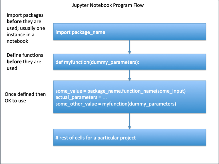
Program Flow and Prototyping¶

A function, whether built-in, or added must be defined before it is called, otherwise the script will fail. Certain built-in functions “self define” upon start (such as print() and type() and we need not worry about those funtions). The diagram below illustrates the requesite flow control for functions that need to be defined before use.

An example below will illustrate, change the cell to code and run it, you should get an error. Then fix the indicated line (remove the leading “#” in the import math … line) and rerun, should get a functioning script.

# reset the notebook using a magic function in JupyterLab
%reset -f 
# An example, run once as is then activate indicated line, run again - what happens?
x= 4.
sqrt_by_arithmetic = x**0.5
print('Using arithmetic square root of ', x, ' is ',sqrt_by_arithmetic )
# import math # import the math package ## activate and rerun
sqrt_by_math = math.sqrt(x)  # note the dot notation
print('Using math package square root of ',  x,' is ',sqrt_by_arithmetic)

An alternate way to load just the sqrt() function is shown below, either way is fine.

# reset the notebook using a magic function in JupyterLab 
%reset -f 
# An example, run once as is then activate indicated line, run again - what happens?
x= 4.
sqrt_by_arithmetic = x**0.5
print('Using arithmetic square root of ', x, ' is ',sqrt_by_arithmetic )
from math import sqrt # import sqrt from the math package ## activate and rerun
sqrt_by_math = sqrt(x)  # note the notation
print('Using math package square root of ',  x,' is ',sqrt_by_arithmetic)

Using arithmetic square root of  4.0  is  2.0
Using math package square root of  4.0  is  2.0

Built-In in Primitive Python (Base install)¶

The base Python functions and types built into it that are always available, the figure below lists those functions.

Notice all have the structure of function_name(), except __import__() which has a constructor type structure, and is not intended for routine use (among other things it allows assigning multiple names for an imported module which usually breaks things badly) but instead we should stick with plain old import module_name as an expression rather than a function call.

Added-In using External Packages/Modules and Libaries (e.g. math)¶

Python is also distributed with a large number of external functions. These functions are saved in files known as modules. To use the built-in codes in Python modules, we have to import them into our programs first. We do that by using the import keyword. There are three ways to import:

Import the entire module by writing import moduleName; For instance, to import the random module, we write import random. To use the randrange() function in the random module, we write random.randrange( 1, 10);28
Import and rename the module by writing import random as r (where r is any name of your choice). Now to use the randrange() function, you simply write r.randrange(1, 10); and
Import specific functions from the module by writing from moduleName import name1[,name2[, … nameN]]. For instance, to import the randrange() function from the random module, we write from random import randrange. To import multiple functions, we separate them with a comma. To import the randrange() and randint() functions, we write from random import randrange, randint. To use the function now, we do not have to use the dot notation anymore. Just write randrange( 1, 10).

# Example 1 of import
%reset -f 
import random
low = 1 ; high = 10
random.randrange(low,high) #generate random number in range low to high

# Example 2 of import
%reset -f 
import random as r
low = 1 ; high = 10
r.randrange(low,high)

# Example 3 of import
%reset -f 
from random import randrange 
low = 1 ; high = 10
randrange(low,high)

The modules that come with Python are extensive and listed at https://docs.python.org/3/py-modindex.html. There are also other modules that can be downloaded and used (just like user defined modules below). In these labs we are building primitive codes to learn how to code and how to create algorithms. For many practical cases you will want to load a well-tested package to accomplish the tasks.

That exercise is saved for the end of the document.

User-Built¶

We can define our own functions in Python and reuse them throughout the program. The syntax for defining a function is:

def functionName( argument ):
    code detailing what the function should do
    note the colon above and indentation
    ...
    ...
    return [expression]

The keyword def tells the program that the indented code from the next line onwards is part of the function. The keyword return tells the program to return an answer from the function. There can be multiple return statements in a function. Once the function executes a return statement, the program exits the function and continues with its next executable statement. If the function does not need to return any value, you can omit the return statement, the exit code will be none which is a special constant with logical value false

Its probably a good habit to have a return statement anyway, and just return null

Functions can be pretty elaborate; they can search for things in a list, determine variable types, open and close files, read and write to files.

To get started we will build a few really simple mathematical functions; we will need this skill in the future anyway, especially in scientific programming contexts.

User-built within a Code Block¶

For our first function we will code

\[f(x) = x\sqrt{1 + x}\]

into a function named dusty().

When you run the next cell, all it does is prototype the function (defines it), nothing happens until we use the function.

def dusty(x) :
    temp = x * ((1.0+x)**(0.5)) # don't need the math package
    return temp
# the function should make the evaluation
# store in the local variable temp
# return contents of temp

When we run the cell above, it seems like nuttin happens - but in fact the kernel (Sanders himself) associates the name dusty with the block of code that we just created. Now we can use the dusty funcrtion at our leisure as below:

# wrapper to run the dusty function
yes = 0
while yes == 0:
    xvalue = input('enter a numeric value')
    try:
        xvalue = float(xvalue)
        yes = 1
    except:
        print('enter a bloody number! Try again \n')
# call the function, get value , write output
yvalue = dusty(xvalue)
print('f(',xvalue,') = ',yvalue) # and we are done 

Example¶

Sum of numbers from 0 to N

def sum_of_n(n):
    mysum = 0 # initialize the accumulator
    for i in range(n+1): # construct an accumulation loop
        mysum = mysum + i
    return mysum

how_many = 4
print(sum_of_n(how_many))

Example¶

Sum of numbers from 0 to N, but forget the return statement

def sum_of_n(n):
    mysum = 0 # initialize the accumulator
    for i in range(n+1): # construct an accumulation loop
        mysum = mysum + i

how_many = 4
print(sum_of_n(how_many))

None

Example¶

Sum of numbers from 0 to N, and including defaults.

def sum_of_n(n=3):
    mysum = 0 # initialize the accumulator
    for i in range(n+1): # construct an accumulation loop
        mysum = mysum + i
    return mysum

print(sum_of_n()) # if we have no argument, uses the default

Example¶

Create a Fahrenhiet to Celsius converter and test it for these values:

32
15
100

*hint: Formula-(°F − 32) × 5/9 = °C

Problem Solving Process¶

Step 1¶

Define the problem (problem statement):

Create a tool to convert Fahrenhiet to Celsius

Step 2¶

Gather information (identify known and unknown values, and governing equations)

Known: Input in F
Unknown: Output in C
Governing Principles: Formula: (°F − 32) × 5/9 = °C

Step 3¶

Generate and evaluate potential solutions

-40F = -40C
32F = 0C
212F = 100C

Step 4¶

Refine and implement a solution

Create function to evaluate input and produce output

def FC(x) : # convert F to C
    C = (x - 32)*5/9
    return C

Create wrapper to prompt for input, execute function, label output

print(FC(99))

37.22222222222222

Step 5¶

Verify and test the solution.

print(FC(-40))

-40.0

print(FC(32))

0.0

print(FC(212))

100.0

Step 6¶

Refine to be useful

Modify the wrapper to be interactive

def F2C(x) : # convert F to C
    C = (x - 32)*5/9
    return C
# wrapper to run the F2C function
yes = 0
while yes == 0:
    xvalue = input('Enter a temperature in Fairyheight')
    try:
        xvalue = float(xvalue)
        yes = 1
    except:
        print('Enter a bloody number! Try again \n')
# call the function, get value , write output
yvalue = F2C(xvalue)
print('Temp: ',xvalue,'F = ',yvalue,' C') # and we are done 

Variable Scope¶

An important concept when defining a function is the concept of variable scope. Variables defined inside a function are treated differently from variables defined outside. Firstly, any variable declared within a function is only accessible within the function. These are known as local variables.

In the dusty() function, the variables x and temp are local to the function. Any variable declared outside a function in a main program is known as a program variable and is accessible anywhere in the program.

In the example, the variables xvalue and yvalue are program variables (global to the program; if they are addressed within a function, they could be operated on.) Generally we want to protect the program variables from the function unless the intent is to change their values. The way the function is written in the example, the function cannot damage xvalue or yvalue.

If a local variable shares the same name as a program variable, any code inside the function is accessing the local variable. Any code outside is accessing the program variable

As Separate Module/File¶

In this section we will invent the neko() function, export it to a file, so we can reuse it in later notebooks without having to retype or cut-and-paste. The neko() function evaluates:

\[f(x) = x\sqrt{|(1 + x)|}\]

Its the same as the dusty() function, except operates on the absolute value in the wadical.

Create a text file named “mylibrary.txt”

Copy the neko() function script below into that file.

 def neko(input_argument) :
     import math #ok to import into a function
     local_variable = input_argument * math.sqrt(abs(1.0+input_argument))
     return local_variable

rename mylibrary.txt to mylibrary.py
modify the wrapper script to use the neko function as an external module

# wrapper to run the neko function
import mylibrary
yes = 0
while yes == 0:
    xvalue = input('enter a numeric value')
    try:
        xvalue = float(xvalue)
        yes = 1
    except:
        print('enter a bloody number! Try again \n')
# call the function, get value , write output
yvalue = mylibrary.neko(xvalue)
print('f(',xvalue,') = ',yvalue) # and we are done 

In JupyterHub environments, you may discover that changes you make to your external python file are not reflected when you re-run your script; you need to restart the kernel to get the changes to actually update. The figure below depicts the notebook, external file relatonship

Future version - explain absolute path

Recursion¶

Functions can contain themselves as part of definition, this is called recursion. Use the provilige with care, its easy to clobber the memory stack using recursive structures. Consider the factorial function definition from math class:

\[\begin{split} 0! = 1 \\ 1! = 1 \\ 2! = 0! * 1! * 2 \\ \dots \\ N! = (N-1)! * N \end{split}\]

def factorial(n=0):
    if n <= 1:
        return 1
    else:
        return n*factorial(n-1)

factorial(6)

Rudimentary Graphics¶

Graphing values is part of the broader field of data visualization, which has two main goals:

To explore data, and
To communicate data.

In this subsection we will concentrate on introducing skills to start exploring data and to produce meaningful visualizations we can use throughout the rest of this notebook. Data visualization is a rich field of study that fills entire books. The reason to start visualization here instead of elsewhere is that with mathematical functions plotting is a natural activity and we have to import the matplotlib module to make the plots.

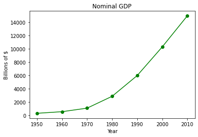
The example below is code adapted from Grus (2015) that illustrates simple generic plots. I added a single line (label the x-axis), and corrected some transcription errors (not the original author’s mistake, just the consequence of how the API handled the cut-and-paste), but otherwise the code is unchanged.

# python script to illustrate plotting
# CODE BELOW IS ADAPTED FROM:
# Grus, Joel (2015-04-14). Data Science from Scratch: First Principles with Python
# (Kindle Locations 1190-1191). O'Reilly Media. Kindle Edition. 
#
import matplotlib.pyplot # import the plotting library from matplotlib.pyplot
# build a couple of lists
years = [1950, 1960, 1970, 1980, 1990, 2000, 2010]  # define one list for years
gdp = [300.2, 543.3, 1075.9, 2862.5, 5979.6, 10289.7, 14958.3] # and another one for Gross Domestic Product (GDP)
# build the plot
matplotlib.pyplot.plot( years, gdp, color ='green', marker ='o', linestyle ='solid') # create a line chart, years on x-axis, gdp on y-axis
                                                                       # what if "^", "P", "*" for marker?
                                                                       # what if "red" for color?  
                                                                       # what if "dashdot", '--' for linestyle?  
matplotlib.pyplot.title("Nominal GDP")# add a title
matplotlib.pyplot.ylabel("Billions of $")# add a label to the x and y-axes
matplotlib.pyplot.xlabel("Year")# add a title
matplotlib.pyplot.show() # display the plot

Now lets put the plotting script into a function so we can make line charts of any two numeric lists

def plotAline(list1,list2,strx,stry,strtitle): # plot list1 on x, list2 on y, xlabel, ylabel, title
    import matplotlib.pyplot # import the plotting library from matplotlib.pyplot
    matplotlib.pyplot.plot( list1, list2, color ='green', marker ='o', linestyle ='solid') # create a line chart, years on x-axis, gdp on y-axis
    matplotlib.pyplot.title(strtitle)# add a title
    matplotlib.pyplot.ylabel(stry)# add a label to the x and y-axes
    matplotlib.pyplot.xlabel(strx)
    matplotlib.pyplot.show() # display the plot
    return #null return

# wrapper script
years = [1950, 1960, 1970, 1980, 1990, 2000, 2010]  # define two lists years and gdp
gdp = [300.2, 543.3, 1075.9, 2862.5, 5979.6, 10289.7, 14958.3]
print(type(years[0]))
print(type(gdp[0]))
plotAline(years,gdp,"Year","Billions of $","Nominal GDP")

<class 'int'>
<class 'float'>

Example¶

Use the plotting script and create a function that draws a straight line between two points. We will cut-and-paste in class to see what this code does for us.

def MakeALine():
    import matplotlib.pyplot # import the plotting library from matplotlib.pyplot
    x1 = input('Please enter x value for point 1')
    y1 = input('Please enter y value for point 1')
    x2 = input('Please enter x value for point 2')
    y2 = input('Please enter y value for point 2')
    xlist = [x1,x2]
    ylist = [y1,y2]
    matplotlib.pyplot.plot( xlist, ylist, color ='orange', marker ='*', linestyle ='solid') 
    #plt.title(strtitle)# add a title
    matplotlib.pyplot.ylabel("Y-axis")# add a label to the x and y-axes
    matplotlib.pyplot.xlabel("X-axis")
    matplotlib.pyplot.show() # display the plot
    return #null return

MakeALine()

References¶

Grus, Joel (2015-04-14). Data Science from Scratch: First Principles with Python (Kindle Locations 1190-1191). O’Reilly Media. Kindle Edition.
Call Expressions in “Adhikari, A. and DeNero, J. Computational and Inferential Thinking The Foundations of Data Science” https://www.inferentialthinking.com/chapters/03/3/Calls.html
Functions and Tables in “Adhikari, A. and DeNero, J. Computational and Inferential Thinking The Foundations of Data Science” https://www.inferentialthinking.com/chapters/08/Functions_and_Tables.html
Visualization in “Adhikari, A. and DeNero, J. Computational and Inferential Thinking The Foundations of Data Science” https://www.inferentialthinking.com/chapters/07/Visualization.html
Documentation; The Python Standard Library; 9. Numeric and Mathematical Modules https://docs.python.org/2/library/math.html
Code.org; Chris Bosh of Miami Heat and Jess Lee CEO of Polyvore. Let’s use code to join Anna and Elsa as they explore the magic and beauty of ice. https://youtu.be/0eo0ESEX9DE

Laboratory 6¶

Examine (click) Laboratory 0 as a webpage at Laboratory 6.html

Download (right-click, save target as …) Laboratory 6 as a jupyterlab notebook from Laboratory 6.ipynb

Exercise Set 6¶

Examine (click) Exercise Set 6 as a webpage at Exercise 6.html

Download (right-click, save target as …) Exercise Set 6 as a jupyterlab notebook at Exercise Set 6.ipynb

ENGR 1330 Course Notes

ENGR 1330 Computational Thinking with Data Science

6: Functions¶

Objectives¶

What are Functions?¶

Calling the Function¶

Program Flow and Prototyping¶

Built-In in Primitive Python (Base install)¶

Added-In using External Packages/Modules and Libaries (e.g. math)¶

User-Built¶

User-built within a Code Block¶

Example¶

Example¶

Example¶

Example¶

Problem Solving Process¶

Step 1¶

Step 2¶

Step 3¶

Step 4¶

Step 5¶

Step 6¶

Variable Scope¶

As Separate Module/File¶

Recursion¶

Rudimentary Graphics¶

Example¶

References¶

Laboratory 6¶

Exercise Set 6¶