ENGR 1330 Computational Thinking with Data Science
Copyright © 2021 Theodore G. Cleveland and Farhang Forghanparast
Last GitHub Commit Date:
32: Logistic Regression
Concept of …
Training (a model fitting analog)
Warning
This lesson is under construction, the scripts work, but narrative is incomplete.
Background
Single Variable Models
Future lesson
Multiple Variable Models
Logistic regression is trying to fit the following data model:
where;
The matrix has as many rows as observations to fit, and as many columns as predictor variables.
Fitting Process
The logistic regression method attempts to find values of \(\beta\) that maximizes the log-likelihood function
The presence of the last term makes the process a search process (instead of a single equation to solve), and some form of iterative least squares is employed - techniques are complex, so in general we rely on packages to handle this work - an illustrative example follows:
Consider a database of 20,000 observations of two predictors \(X1\) and \(X2\), and the resulting classification \(Class\). We can employ logistic regression to find values of \(/beta\) in the above models, then use those values to predict the classification of a new input.
Step 1 Load packages
Read the database
import pandas as pd
import numpy as np
import sklearn.metrics as metrics
import matplotlib.pyplot as plt
import seaborn as sns
%matplotlib inline
Step 2 Read the database
A copy is located here
mydatabase = pd.read_csv('LogisticRegressionHomebrewExample.csv')
Step 3 Verify the read, and plot the database
mydatabase.describe()
| X1 | X2 | Class | |
|---|---|---|---|
| count | 20000.000000 | 20000.000000 | 20000.000000 |
| mean | 0.496920 | 2.001764 | 0.500000 |
| std | 1.113666 | 2.240266 | 0.500013 |
| min | -4.214002 | -3.489115 | 0.000000 |
| 25% | -0.260873 | -0.015846 | 0.000000 |
| 50% | 0.498444 | 1.978725 | 0.500000 |
| 75% | 1.264066 | 4.016432 | 1.000000 |
| max | 4.605613 | 7.945987 | 1.000000 |
#Split dataframe based on class value and plot
classzero = mydatabase[mydatabase['Class']<1.0]
classone = mydatabase[mydatabase['Class']>0.0]
# plot the two classes as red and blue
plt.figure(figsize=(10, 8))
plt.scatter(classzero['X1'],classzero['X2'], c="red", alpha=0.3)
plt.scatter(classone['X1'],classone['X2'], c="blue", alpha=0.3)
plt.legend(["Class 0","Class 1"])
plt.xlabel('X1 Predictor')
plt.ylabel('X2 Predictor')
plt.grid(which='both')
plt.show()

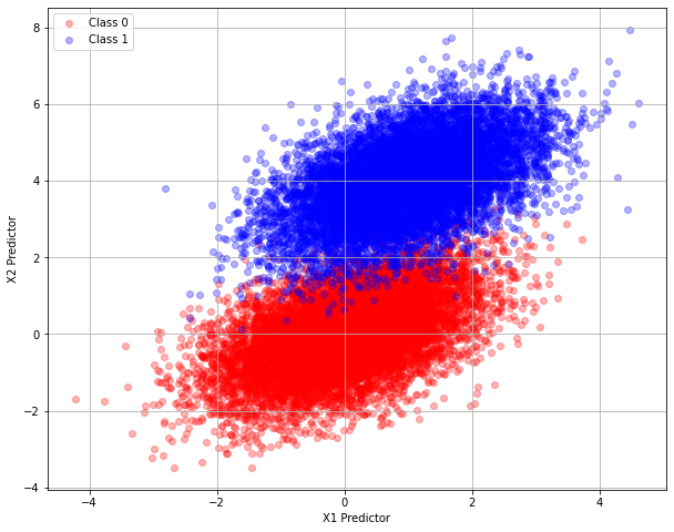
The two classes appear different enough so the logistic-regression classification seems possible. For example if the predictor input is \([0,0]\) then the class is likely “Class 0”, whereas if the predictor input is \([0,4]\) then the class is likely “Class 1” according to the above plot.
Step 4 Employ sklearn to obtain a logistic regresion model
Here we use a package to actually pass a classification boundary between the two data clouds
Prepare the Data to feed into sklearn
#split dataset in features and target variable
feature_cols = ['X1', 'X2']
X = mydatabase[feature_cols] # Features
y = mydatabase["Class"] # Target variable
# split X and y into training and testing sets
from sklearn.model_selection import train_test_split
X_train,X_test,y_train,y_test=train_test_split(X,y,test_size=0.25,random_state=0)
# import the class
from sklearn.linear_model import LogisticRegression

# instantiate the model (using the default parameters)
#logreg = LogisticRegression()
logreg = LogisticRegression()
# fit the model with data
logreg.fit(X_train,y_train)

#
y_pred=logreg.predict(X_test)
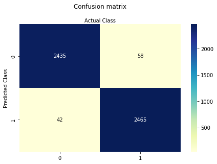
Step 5 Assess the fitted results using a confusion matrix
Compute the matrix, then render using a heat map style.
# import the metrics class
from sklearn import metrics
cnf_matrix = metrics.confusion_matrix(y_pred, y_test)
#cnf_matrix
class_names=[0,1] # name  of classes
fig, ax = plt.subplots()
tick_marks = np.arange(len(class_names))
plt.xticks(tick_marks, class_names)
plt.yticks(tick_marks, class_names)
# create heatmap
sns.heatmap(pd.DataFrame(cnf_matrix), annot=True, cmap="YlGnBu" ,fmt='g')
ax.xaxis.set_label_position("top")
plt.tight_layout()
plt.title('Confusion matrix', y=1.1)
plt.ylabel('Predicted Class')
plt.xlabel('Actual Class');

Step 6 Build a Classifer Engine
Now lets build a classification (class prediction) engine using logistic regression results.
First we need the sigmoid response function where
def sigmoid(scores): # scores = b0+b1X1+b2X2+... where b0,b1,b2,... are specified
    return 1/(1+np.exp(-scores))
Employ the Classifier Engine
Now lets use our two obvious values from the discussion above
inputs = np.array([[0],[0]]) # one example input, should evaluate as
scores = np.dot(logreg.coef_,inputs) + logreg.intercept_
estimated_class = sigmoid(np.dot(logreg.coef_,inputs) + logreg.intercept_)[0,0] # grab the only element
print("X1 Input = ",inputs[0][0],"\nX2 Input = ",inputs[1][0],"\nEstimated Class Value",round(estimated_class,0))
X1 Input =  0
X2 Input =  0
Estimated Class Value 0.0
inputs = np.array([[0],[4]]) # one example input, should evaluate as
scores = np.dot(logreg.coef_,inputs) + logreg.intercept_
estimated_class = sigmoid(np.dot(logreg.coef_,inputs) + logreg.intercept_)[0,0] # grab the only element
print("X1 Input = ",inputs[0][0],"\nX2 Input = ",inputs[1][0],"\nEstimated Class Value",round(estimated_class,0))
X1 Input =  0
X2 Input =  4
Estimated Class Value 1.0
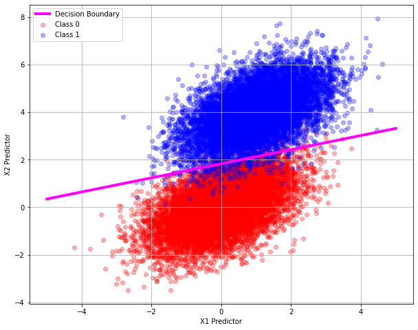
So now we have a classifer function, we could probably draw a dividing line back on the original plot and identify the dividing line, we only need two points where the classifier returns a value of 0.5 as below
inputs = np.array([[-5],[0.347]]) # one example input, should evaluate as
scores = np.dot(logreg.coef_,inputs) + logreg.intercept_
estimated_class = 1.0 - sigmoid(np.dot(logreg.coef_,inputs) + logreg.intercept_)[0,0] # grab the only element
print("X1 Input = ",inputs[0][0],"\nX2 Input = ",inputs[1][0],"\nEstimated Class Value",round(estimated_class,3))
X1 Input =  -5.0
X2 Input =  0.347
Estimated Class Value 0.5
inputs = np.array([[5],[3.314]]) # one example input, should evaluate as
scores = np.dot(logreg.coef_,inputs) + logreg.intercept_
estimated_class = 1.0 - sigmoid(np.dot(logreg.coef_,inputs) + logreg.intercept_)[0,0] # grab the only element
print("X1 Input = ",inputs[0][0],"\nX2 Input = ",inputs[1][0],"\nEstimated Class Value",round(estimated_class,3))
X1 Input =  5.0
X2 Input =  3.314
Estimated Class Value 0.5
Our two points by trial and error are: \([-5.0,0.347]\) and \([5.0,3.314]\) we can add this line to our plot
# plot the two classes as red and blue
plt.figure(figsize=(10, 8))
plt.plot([-5,5],[0.347,3.314],c="magenta",linewidth=4)
plt.scatter(classzero['X1'],classzero['X2'], c="red", alpha=0.3)
plt.scatter(classone['X1'],classone['X2'], c="blue", alpha=0.3)
plt.legend(["Decision Boundary","Class 0","Class 1"])
plt.xlabel('X1 Predictor')
plt.ylabel('X2 Predictor')
plt.grid(which='both')
plt.show()

