
ENGR 1330 Computational Thinking with Data Science
Copyright © 2021 Theodore G. Cleveland and Farhang Forghanparast
Last GitHub Commit Date: 31 January 2021
18: Causality, Correlation, Randomness, and Probability
Concept of causality and correlation (compare and contrast)
Randomness (a prelude to simulation)
Objectives
To understand the fundamental concepts involved in causality; and the difference between cause and correlation.
To understand the fundamental concepts involved in simulation.
To apply concepts involved in iteration.
Computational Thinking Concepts
Causality, Iteration, Simulation =>
Algorithm DesignIteration, Simulation =>
Create Computational Models
Correlation and Causality
What is causality? (A long winded psuedo definition!)
Causality is the relationship between causes and effects. The notion of causality does not have a uniform definition in the sciences, and is studied using philosophy and statistics. From the perspective of physics, it is generally believed that causality cannot occur between an effect and an event that is not in the back (past) light cone of said effect. Similarly, a cause could not have an effect outside its front (future) light cone.
Here are some recent articles regarding Closed Time Loops, that explains causal consistency. The second paper is by an undergraduate student!
Both to some extent theoretically support our popular notion of time travel (aka Dr. Who) without pesky paradoxes; someone with creative writing juices, could have a good science fiction career using these papers as a starting thesis!
In classical physics, an effect cannot occur before its cause. In Einstein’s theory of special relativity, causality means that an effect can not occur from a cause that is not in the back (past) light cone of that event. Similarly, a cause cannot have an effect outside its front (future) light cone. These restrictions are consistent with the assumption that causal influences cannot travel faster than the speed of light and/or backwards in time. In quantum field theory, observables of events with a spacelike relationship, “elsewhere”, have to commute, so the order of observations or measurements of such observables do not impact each other.
Causality in this context should not be confused with Newton’s second law, which is related to the conservation of momentum, and is a consequence of the spatial homogeneity of physical laws. The word causality in this context means that all effects must have specific causes.
Another requirement, at least valid at the level of human experience, is that cause and effect be mediated across space and time (requirement of contiguity). This requirement has been very influential in the past, in the first place as a result of direct observation of causal processes (like pushing a cart), in the second place as a problematic aspect of Newton’s theory of gravitation (attraction of the earth by the sun by means of action at a distance) replacing mechanistic proposals like Descartes’ vortex theory; in the third place as an incentive to develop dynamic field theories (e.g., Maxwell’s electrodynamics and Einstein’s general theory of relativity) restoring contiguity in the transmission of influences in a more successful way than in Descartes’ theory.
Yada yada bla bla bla …
Correlation (Causality’s mimic!)
The literary (as in writing!) formulation of causality is a “why?, because …” structure (sort of like if=>then) The answer to a because question, should be the “cause.” Many authors use “since” to imply cause, but it is incorrect grammar - since answers the question of when?
Think “CAUSE” => “EFFECT”
Correlation doesn’t mean cause (although it is a really good predictor of the crap we all buy - its why Amazon is sucessfull)
Consider the chart below
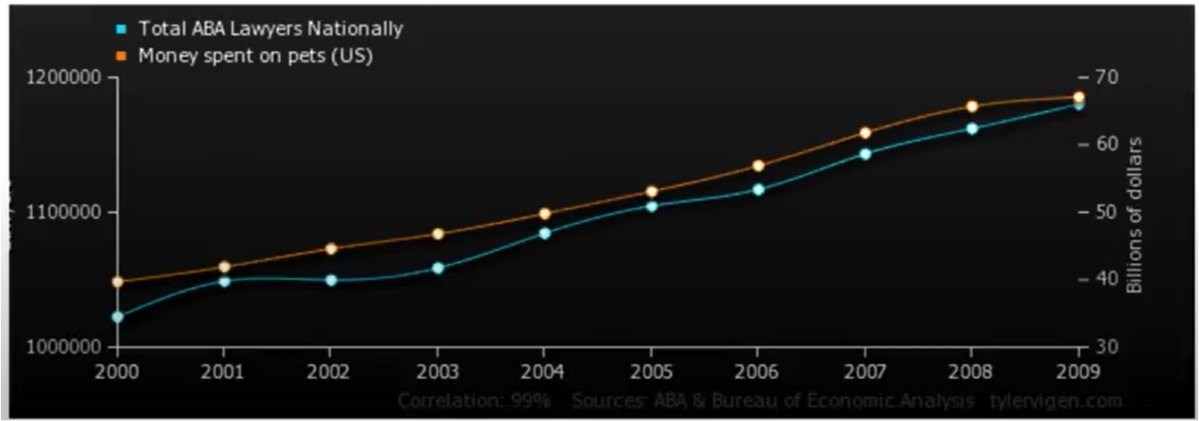
The correlation between money spent on pets and the number of lawyers is quite good (nearly perfect), so does having pets cause lawyers? Of course not, the general social economic conditions that improve general wealth, and create sufficient disposable income to have pets (here we mean companion animals, not food on the hoof) also creates conditions for laywers to proliferate, hence a good correlation.
Nice video : Correlation and Causation https://www.youtube.com/watch?v=1Sa2v7kVEc0
Taking some cues from http://water.usgs.gov/pubs/twri/twri4a3/
Concentrations of atrazine and nitrate in shallow groundwaters are measured in wells over a several county area. For each sample, the concentration of one is plotted versus the concentration of the other. As atrazine concentrations increase, so do nitrate. How might the strength of this association be measured and summarized?
Streams draining the Sierra Nevada mountains in California usually receive less precipitation in November than in other months. Has the amount of November precipitation significantly changed over the last 70 years, showing a gradual change in the climate of the area? How might this be tested?
The above situations require a measure of the strength of association between two continuous variables, such as between two chemical concentrations, or between amount of precipitation and time. How do they co-vary? One class of measures are called correlation coefficients.
Also important is how the significance of that association can be tested for, to determine whether the observed pattern differs from what is expected due entirely to chance.
Whenever a correlation coefficient is to be calculated, the data should be plotted on a scatterplot. No single numerical measure can substitute for the visual insight gained from a plot. Many different patterns can produce the same correlation coefficient, and similar strengths of relationships can produce differing coefficients, depending on the curvature of the relationship.
Association Measures (Covariance and Correlation)
Covariance: is a measure of the joint variability of two random variables. The formula to compute covariance is:
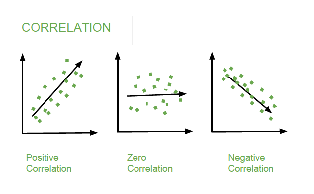
If the greater values of one variable mainly correspond with the greater values of the other variable, and the same holds for the lesser values, (i.e., the variables tend to show similar behavior), the covariance is positive. In the opposite case, when the greater values of one variable mainly correspond to the lesser values of the other, (i.e., the variables tend to show opposite behavior), the covariance is negative. The sign of the covariance therefore shows the tendency of any linear relationship between the variables. The magnitude of the covariance is not particularly useful to interpret because it depends on the magnitudes of the variables.
A normalized version of the covariance, the correlation coefficient, however, is useful in terms of sign and magnitude.
Correlation Coefficient: is a measure how strong a relationship is between two variables. There are several types of correlation coefficients, but the most popular is Pearson’s. Pearson’s correlation (also called Pearson’s R) is a correlation coefficient commonly used in linear regression. Correlation coefficient formulas are used to find how strong a relationship is between data. The formula for Pearson’s R is:
The correlation coefficient returns a value between -1 and 1, where:
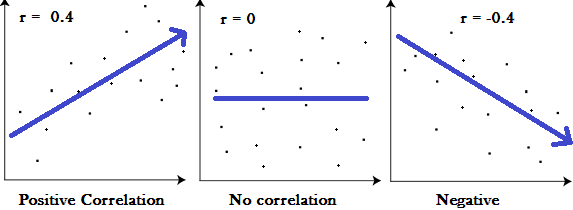
1 : A correlation coefficient of 1 means that for every positive increase in one variable, there is a positive increase of a fixed proportion in the other. For example, shoe sizes go up in (almost) perfect correlation with foot length.
-1: A correlation coefficient of -1 means that for every positive increase in one variable, there is a negative decrease of a fixed proportion in the other. For example, the amount of gas in a tank decreases in (almost) perfect correlation with speed.
0 : Zero means that for every increase, there isn’t a positive or negative increase. The two just aren’t related.
A simple example should illustrate the concept of association
Consider a table of recorded times and speeds from some experimental observations:
Elapsed Time (s) |
Speed (m/s) |
|---|---|
0 |
0 |
1.0 |
3 |
2.0 |
7 |
3.0 |
12 |
4.0 |
20 |
5.0 |
30 |
6.0 |
45.6 |
7.0 |
60.3 |
8.0 |
77.7 |
9.0 |
97.3 |
10.0 |
121.1 |
Create a dataframe:
# Load the necessary packages
import numpy as np
import pandas as pd
import statistics # this package contains correlation and covariance, so we don't have to write code
from matplotlib import pyplot as plt

# Create a dataframe:
time = [0, 1.0, 2.0, 3.0, 4.0, 5.0, 6.0, 7.0, 8.0, 9.0, 10.0]
speed = [0, 3, 7, 12, 20, 30, 45.6, 60.3, 77.7, 97.3, 121.2]
data = pd.DataFrame({'Time':time, 'Speed':speed})
data
| Time | Speed | |
|---|---|---|
| 0 | 0.0 | 0.0 |
| 1 | 1.0 | 3.0 |
| 2 | 2.0 | 7.0 |
| 3 | 3.0 | 12.0 |
| 4 | 4.0 | 20.0 |
| 5 | 5.0 | 30.0 |
| 6 | 6.0 | 45.6 |
| 7 | 7.0 | 60.3 |
| 8 | 8.0 | 77.7 |
| 9 | 9.0 | 97.3 |
| 10 | 10.0 | 121.2 |
Now, let’s explore the data:
data.describe()
| Time | Speed | |
|---|---|---|
| count | 11.000000 | 11.000000 |
| mean | 5.000000 | 43.100000 |
| std | 3.316625 | 41.204077 |
| min | 0.000000 | 0.000000 |
| 25% | 2.500000 | 9.500000 |
| 50% | 5.000000 | 30.000000 |
| 75% | 7.500000 | 69.000000 |
| max | 10.000000 | 121.200000 |
time_var = statistics.variance(time)
speed_var = statistics.variance(speed)

print("Variance of recorded times is ",time_var)
print("Variance of recorded times is ",speed_var)
Variance of recorded times is  11.0
Variance of recorded times is  1697.7759999999998
Is there evidence of a relationship (based on covariance, correlation) between time and speed?
# To find the covariance
data.cov()
| Time | Speed | |
|---|---|---|
| Time | 11.00 | 131.750 |
| Speed | 131.75 | 1697.776 |
# To find the correlation among the columns
# using pearson method
data.corr(method ='pearson')
| Time | Speed | |
|---|---|---|
| Time | 1.000000 | 0.964082 |
| Speed | 0.964082 | 1.000000 |
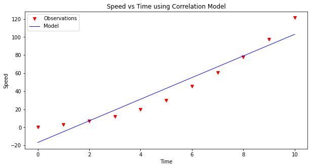
These values suggest that time, \(t\), is a good estimator of time (correlation is perfect as anticipated), and also a good estimator of speed, \(u\), (nearly perfect).
We can hack a useable linear model as:
\(u \approx \bar u + (cov(u,t)/cov(t,t))(t-\bar t)\)
And assess the model by plotting
import matplotlib.pyplot as plt
def make2plot(listx1,listy1,listx2,listy2,strlablx,strlably,strtitle):
    mydata = plt.figure(figsize = (10,5)) # build a square drawing canvass from figure class
    plt.plot(listx1,listy1, c='red', marker='v',linewidth=0) # basic data plot
    plt.plot(listx2,listy2, c='blue',linewidth=1) # basic model plot
    plt.xlabel(strlablx)
    plt.ylabel(strlably)
    plt.legend(['Observations','Model'])# modify for argument insertion
    plt.title(strtitle)
    plt.show()
    return
model = data['Speed'].mean()+(data['Time']-data['Time'].mean())*(data.cov().iloc[1,0]/data.cov().iloc[0,0] )
make2plot(data['Time'],data['Speed'],data['Time'],model,'Time','Speed','Speed vs Time using Correlation Model')
Implications
Most research questions attempt to explain cause and effect.
In experimental research, the relationship is constructed and the experiment is somewhat of a failure if none of the presumed causal (causal == explainatory) variables influence the response (response == effect)
In a data science experimental context, causality may be impossible to establish, however correlations can be established and exploited.
In data science, many studies involve observations on a group of individuals, a factor of interest called a treatment (explainatory variable, predictor variable, predictor feature …), and an outcome (response, effect, state, predicted value …) measured on each individual.
The presumptive establishment of causality takes place in two stages.
First, an association is observed. Any relation between the treatment and the outcome is called an association (we can measure the strength of the association using correlation coefficients!).
Second, A more careful analysis is used to establish causality.
One approach would be to control all variables other than the suspected (explainatory) variables, which for any meaningful process is essentially impossible.
Another approach is to establish randomized control studies:
Start with a sample from a population (e.g. volunteers to test Covid 19 vaccines)
Randomly assign members to either 1. Control group 2. Treatment group
Expose the two groups identically, except the control group recieves a false (null) treatment
Compare the responses of the two groups, if they are same, there exists no evidence that the treatment variable CAUSES a response
These concepts can be extended with some ingenuity to engineered systems and natural systems.
Consider

Data Science Questions:
Does going to school cause flu?
Does flu cause school attendance?
Does going to school contribute to the spread of flu?
Does the spread of flu contribute to the school attendance?
Are there other variables that affects both?
a. These are called “confounding factors” or “lurking variables”.
b. Cold weather?, more indoor time?, more interaction?
Confounding Factors
An underlying difference between the two groups (other than the treatment) is called a confounding factor, because it might confound you (that is, mess you up) when you try to reach a conclusion.
For example, Cold weather in the previous example.
Confounding also occurs when explainatory variables are correlated to another, for instance flood flows are well correlated to drainage area, main channel length, mean annual precipitation, main channel slope, and elevation. However main channel length is itself strongly correlated to drainage area, so much so as to be nearly useless as an explainatory variable when drainage area is retained in a data model. It would be a “confounding variable” in this context.
Randomization
To establish presumptive causality in data science experiments, we need randomization tools.
We can use Python to make psuedo-random choices.
There are built-in functions in numpy library under random submodule.
The choice function randomly picks one item from an array.
The syntax is
np.random.choice(array_name), where array_name is the name of the array from which to make the choice.
#Making Random Choice from an Array (or list)
import numpy as np
two_groups = np.array(['treatment', 'control'])
np.random.choice(two_groups,1)
# mylist = ['treatment', 'control']  # this works too
# np.random.choice(mylist)
array(['control'], dtype='<U9')
The difference of this function from others that we learned so far, is that it doesn’t give the same result every time. We can roll a dice using this function by randomly selecting from an array from 1 to 6.
my_die = np.array(['one', 'two','three', 'four','five', 'six'])
np.random.choice(my_die)
'two'
# now a bunch of rolls
print('roll #1 ',np.random.choice(my_die) )
print('roll #2 ',np.random.choice(my_die) )
print('roll #3 ',np.random.choice(my_die) )
print('roll #4 ',np.random.choice(my_die) )
print('roll #5 ',np.random.choice(my_die) )
print('roll #6 ',np.random.choice(my_die) )
roll #1  four
roll #2  two
roll #3  five
roll #4  one
roll #5  three
roll #6  six
# or multiple rolls, single call
myDiceRolls = np.random.choice(my_die,6)
print(myDiceRolls)
['four' 'five' 'five' 'two' 'six' 'six']
We might need to repeat a process multiple times to reach better results or cover more results. Let’s create a game with following rules:
If the dice shows 1 or 2 spots, my net gain is -1 dollar.
If the dice shows 3 or 4 spots, my net gain is 0 dollars.
If the dice shows 5 or 6 spots, my net gain is 1 dollar.
my_wallet = 1 # start with 1 dollars

def place_a_bet(wallet):
    print("Place your bet!")
    if wallet == 0:
        print("You have no money, get out of my Casino!")
        return(wallet)
    else:
        wallet = wallet - 1
        return(wallet)

def make_a_roll(wallet):
    """Returns my net gain on one bet"""
    print("Roll the die!")
    x = np.random.choice(np.arange(1, 7))  # roll a die once and record the number of spots
    if x <= 2:
        print("You Lose,  Bummer!")
        return(wallet) # lose the bet
    elif x <= 4:
        print("You Draw, Take your bet back.")
        wallet = wallet+1
        return(wallet) # draw, get bet back
    elif x <= 6:
        print("You win a dollar!")
        wallet = wallet+2
        return (wallet) # win, get bet back and win a dollar!


# Single play
print("Amount in my account =:",my_wallet)
my_wallet = place_a_bet(my_wallet)
my_wallet = make_a_roll(my_wallet)
print("Amount in my account =:",my_wallet)
Amount in my account =: 1
Place your bet!
Roll the die!
You Draw, Take your bet back.
Amount in my account =: 1
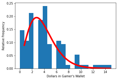
A more automated solution is to use a for statement to loop over the contents of a sequence. Each result is called iteration. Here we use a for statement in a more realistic way: we print the results of betting five times on the die as described earlier. This process is called simulating the results of five bets. We use the word simulating to remind ourselves that we are not physically rolling dice and exchanging money but using Python to mimic the process.
# Some printing tricks
CRED = '\033[91m'
CEND = '\033[0m'

my_wallet = 10
how_many_throws = 1

for i in range(how_many_throws):
    print("Amount in my account =:",my_wallet)
    my_wallet = place_a_bet(my_wallet)
    my_wallet = make_a_roll(my_wallet)

#print(CRED + "Error, does not compute!" + CEND)
    print("After ",i+1," plays")
    print(CRED + "Amount in my account =:",my_wallet,CEND)
    print("_______________________")
Amount in my account =: 10
Place your bet!
Roll the die!
You Draw, Take your bet back.
After  1  plays
Amount in my account =: 10
_______________________
Simulation of multiple gamblers/multiple visits to the Casino
https://www.inferentialthinking.com/chapters/09/3/Simulation.html
outcomes = np.array([])  #null array to store outcomes

# redefine functions to suppress output

def place_a_bet(wallet):
    # print("Place your bet!")
    if wallet == 0:
        # print("You have no money, get out of my Casino!")
        return(wallet)
    else:
        wallet = wallet - 1
        return(wallet)

def make_a_roll(wallet):
    """Returns my net gain on one bet"""
    # print("Roll the die!")
    x = np.random.choice(np.arange(1, 7))  # roll a die once and record the number of spots
    if x <= 2:
        #print("You Lose,  Bummer!")
        return(wallet) # lose the bet
    elif x <= 4:
        #print("You Draw, Take your bet back.")
        wallet = wallet+1
        return(wallet) # draw, get bet back
    elif x <= 6:
        #print("You win a dollar!")
        wallet = wallet+2
        return (wallet) # win, get bet back and win a dollar!


# Some printing tricks
CRED = '\033[91m'
CEND = '\033[0m'


how_many_simulations = 100

for j in range(how_many_simulations):
    my_wallet = 1
    how_many_throws = 30

    for i in range(how_many_throws):
     #   print("Amount in my account =:",my_wallet)
        my_wallet = place_a_bet(my_wallet)
        my_wallet = make_a_roll(my_wallet)

#print(CRED + "Error, does not compute!" + CEND)
#    print("After ",i+1," plays")
#    print(CRED + "Amount in my account =:",my_wallet,CEND)
#    print("_______________________")

    outcomes = np.append(outcomes,my_wallet)

# build a histogram chart - outcomes is an array

import matplotlib.pyplot as plt
from scipy.stats import gamma

#ax.hist(r, density=True, histtype='stepfilled', alpha=0.2)
plt.hist(outcomes, density=True, bins = 20)
plt.xlabel("Dollars in Gamer's Wallet")
plt.ylabel('Relative Frequency')
#### just a data model, gamma distribution ##############
# code below adapted from https://docs.scipy.org/doc/scipy/reference/generated/scipy.stats.gamma.html
a = 5 # bit of trial and error
x = np.linspace(gamma.ppf(0.001, a),gamma.ppf(0.999, a), 1000)
plt.plot(x, gamma.pdf(x, a, loc=-1.25, scale=1),'r-', lw=5, alpha=1.0, label='gamma pdf')
#########################################################
# Render the plot
plt.show()

#print("Expected value of wallet (mean) =: ",outcomes.mean())

import pandas as pd
df = pd.DataFrame(outcomes)
df.describe()
| 0 | |
|---|---|
| count | 100.000000 |
| mean | 4.050000 |
| std | 3.169855 |
| min | 0.000000 |
| 25% | 2.000000 |
| 50% | 4.000000 |
| 75% | 6.000000 |
| max | 15.000000 |
Simulation
Simulation is the process of using a computer to mimic a real experiment or process. In this class, those experiments will almost invariably involve chance.
To summarize from: https://www.inferentialthinking.com/chapters/09/3/Simulation.html
Step 1: What to Simulate: Specify the quantity you want to simulate. For example, you might decide that you want to simulate the outcomes of tosses of a coin.
Step 2: Simulating One Value: Figure out how to simulate one value of the quantity you specified in Step 1. (usually turn into a function for readability)
Step 3: Number of Repetitions: Decide how many times you want to simulate the quantity. You will have to repeat Step 2 that many times.
Step 4: Coding the Simulation: Put it all together in code.
Step 5: Interpret the results (plots,
Simulation Example
Should I change my choice?
Based on Monty Hall example from https://youtu.be/Xp6V_lO1ZKA But we already have a small car! (Also watch https://www.youtube.com/watch?v=6Ewq_ytHA7g to learn significance of the small car!)
Consider

The gist of the game is that a contestent chooses a door, the host reveals one of the unselected doors and offers the contestant a chance to change their choice. Should the contestant stick with her initial choice, or switch to the other door? That is the Monty Hall problem.
Using classical probability theory it is straightforward to show that:
The chance that the car is behind the originally chosen door is 1/3.
After Monty opens the door with the goat, the chance distribution changes.
If the contestant switches the decision, he/she doubles the chance.
Suppose we have harder situations, can we use this simple problem to learn how to ask complex questions?
import numpy as np
import pandas as pd
import matplotlib.pyplot as plt

def othergoat(x):         #Define a function to return "the other goat"!
    if x == "Goat 1":
        return "Goat 2"
    elif x == "Goat 2":
        return "Goat 1"

Doors = np.array(["Car","Goat 1","Goat 2"])     #Define a list for objects behind the doors
goats = np.array(["Goat 1" , "Goat 2"])          #Define a list for goats!

def MHgame():
    #Function to simulate the Monty Hall Game
    #For each guess, return ["the guess","the revealed", "the remaining"]
    userguess=np.random.choice(Doors)         #randomly selects a door as userguess
    if userguess == "Goat 1":
        return [userguess, "Goat 2","Car"]
    if userguess == "Goat 2":
        return [userguess, "Goat 1","Car"]
    if userguess == "Car":
        revealed = np.random.choice(goats)
        return [userguess, revealed,othergoat(revealed)]
# Check and see if the MHgame function is doing what it is supposed to do:
for i in np.arange(1):
    a =MHgame()
    print(a)
    print(a[0])
    print(a[1])
    print(a[2])
['Goat 1', 'Goat 2', 'Car']
Goat 1
Goat 2
Car
c1 = []         #Create an empty list for the userguess
c2 = []         #Create an empty list for the revealed
c3 = []         #Create an empty list for the remaining

how_many_games = 10000

for i in np.arange(how_many_games):         #Simulate the game for 1000 rounds - or any other number of rounds you desire
    game = MHgame()
    c1.append(game[0])             #In each round, add the first element to the userguess list
    c2.append(game[1])             #In each round, add the second element to the revealed list
    c3.append(game[2])             #In each round, add the third element to the remaining list
#Create a data frame (gamedf) with 3 columns ("Guess","Revealed", "Remaining") and 1000 (or how many number of rounds) rows
gamedf = pd.DataFrame({'Guess':c1,
                       'Revealed':c2,
                       'Remaining':c3})
gamedf
| Guess | Revealed | Remaining | |
|---|---|---|---|
| 0 | Goat 1 | Goat 2 | Car |
| 1 | Goat 1 | Goat 2 | Car |
| 2 | Goat 1 | Goat 2 | Car |
| 3 | Goat 1 | Goat 2 | Car |
| 4 | Goat 2 | Goat 1 | Car |
| ... | ... | ... | ... |
| 9995 | Goat 2 | Goat 1 | Car |
| 9996 | Car | Goat 1 | Goat 2 |
| 9997 | Goat 1 | Goat 2 | Car |
| 9998 | Goat 2 | Goat 1 | Car |
| 9999 | Goat 2 | Goat 1 | Car |
10000 rows × 3 columns
# Get the count of each item in the first and 3rd column
original_car =gamedf[gamedf.Guess == 'Car'].shape[0]
remaining_car =gamedf[gamedf.Remaining == 'Car'].shape[0]

original_g1 =gamedf[gamedf.Guess == 'Goat 1'].shape[0]
remaining_g1 =gamedf[gamedf.Remaining == 'Goat 1'].shape[0]

original_g2 =gamedf[gamedf.Guess == 'Goat 2'].shape[0]
remaining_g2 =gamedf[gamedf.Remaining == 'Goat 2'].shape[0]
# Let's plot a grouped barplot

# set width of bar
barWidth = 0.25

# set height of bar
bars1 = [original_car,original_g1,original_g2]
bars2 = [remaining_car,remaining_g1,remaining_g2]

# Set position of bar on X axis
r1 = np.arange(len(bars1))
r2 = [x + barWidth for x in r1]

# Make the plot
plt.bar(r1, bars1, color='darkorange', width=barWidth, edgecolor='white', label='Original Guess')
plt.bar(r2, bars2, color='midnightblue', width=barWidth, edgecolor='white', label='Remaining Door')

# Add xticks on the middle of the group bars
plt.xlabel('Item', fontweight='bold')
plt.xticks([r + barWidth/2 for r in range(len(bars1))], ['Car', 'Goat 1', 'Goat 2'])

# Create legend & Show graphic
plt.legend()
plt.show()
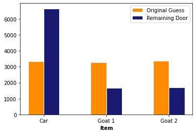
Interpret Results
According to the plot, it is beneficial for the players to switch doors because the initial chance for being correct is only 1/3
Does changing doors have a CAUSAL effect on outcome?
Randomness and Probability
The textbook presents randomness at: https://www.inferentialthinking.com/chapters/09/Randomness.html
Section 9.5 of that link elaborates on probabilities
“Over the centuries, there has been considerable philosophical debate about what probabilities are. Some people think that probabilities are relative frequencies; others think they are long run relative frequencies; still others think that probabilities are a subjective measure of their own personal degree of uncertainty.”
As a practical matter, most probabilities are relative frequencies. If you are a Bayesian statistician, its just conditioned relative frequency. By convention, probabilities are numbers between 0 and 1, or, equivalently, 0% and 100%. Impossible events have probability 0. Events that are certain have probability 1.
As a silly example, the probability that a Great White shark will swim up your sewer pipe and bite you on the bottom, is zero. Unless the sewer pipe is pretty big, the shark cannot physically get to you - hence impossible. Now if you are swimming in a freshwater river, lets say the Columbia river on the Oregon border, that probability of sharkbite increases a bit, perhaps 1 in 100 million, or 0.000001% chance of a Great White shark (a pelagic species adapted to salt water), swimming upriver in freshwater, past a couple of fish ladders, still hungry enough bite your bottom. It would be a rare bite indeed; but not physically impossible.

At the other end of the scale, “sure things” have a probability close to 1. If you run and jump off Glacier point in Yosemite Valley, its almost guarenteed that you will have a 1000 foot plunge until you hit the apron of the cliff and make a big red smear - there could be a gust of wind pushing you away into the trees, but pretty unlikely. So without a squirrel suit and a parachute you are pretty much going to expire with probability 100% chance.
Math is the main tool for finding probabilities exactly, though computers are useful for this purpose too. Simulation can provide excellent approximations. In this section, we will informally develop a few simple rules that govern the calculation of probabilities. In subsequent sections we will return to simulations to approximate probabilities of complex events.
We will use the standard notation 𝑃(event) to denote the probability that “event” happens, and we will use the words “chance” and “probability” interchangeably.
Concepts of sample, population, and probabilities.
Computing probability: single events, both events, at least event.
Simple Exclusion
If the chance that event happens is 40%, then the chance that it doesn’t happen is 60%. This natural calculation can be described in general as follows:
𝑃(an event doesn’t happen) = 1−𝑃(the event happens)
The result is correct if the entireity of possibilities are enumerated, that is the entire population is described.
Complete Enumeration
If you are rolling an ordinary die, a natural assumption is that all six faces are equally likely. Then probabilities of how one roll comes out can be easily calculated as a ratio. For example, the chance that the die shows an even number is
Similarly, $\(𝑃(die~shows~a~multiple~of~3) = \frac{\#{3,6}}{\#{1,2,3,4,5,6}} = \frac{2}{6}\)$
In general, $\(𝑃(an event happens) = \frac{outcomes that make the event happen}{all outcomes}\)$
Provided all the outcomes are equally likely. As above, this presumes the entireity of possibilities are enumerated.
In the case of a single die, there are six outcomes - these comprise the entire population of outcomes. If we roll two die there are 12 outcomes, three die 18 and so on.
Not all random phenomena are as simple as one roll of a die. The two main rules of probability, developed below, allow mathematicians to find probabilities even in complex situations.
Conditioning (Two events must happen)
Suppose you have a box that contains three tickets: one red, one blue, and one green. Suppose you draw two tickets at random without replacement; that is, you shuffle the three tickets, draw one, shuffle the remaining two, and draw another from those two. What is the chance you get the green ticket first, followed by the red one?
There are six possible pairs of colors: RB, BR, RG, GR, BG, GB (we’ve abbreviated the names of each color to just its first letter). All of these are equally likely by the sampling scheme, and only one of them (GR) makes the event happen. So $\( 𝑃(green~first,~then~red) = \frac{GR}{RB, BR, RG, GR, BG, GB} = \frac{1}{6} \)$
But there is another way of arriving at the answer, by thinking about the event in two stages. First, the green ticket has to be drawn. That has chance 1/3, which means that the green ticket is drawn first in about 1/3 of all repetitions of the experiment.
But that doesn’t complete the event. Among the 1/3 of repetitions when green is drawn first, the red ticket has to be drawn next. That happens in about 1/2 of those repetitions, and so:
This calculation is usually written “in chronological order,” as follows.
The factor of $\(\frac{1}{2}\)$ is called ” the conditional chance that the red ticket appears second, given that the green ticket appeared first.”
In general, we have the multiplication rule:
Thus, when there are two conditions – one event must happen, as well as another – the chance is a fraction of a fraction, which is smaller than either of the two component fractions. The more conditions that have to be satisfied, the less likely they are to all be satisfied.
Partitioning (When sequence doesn’t matter) - A kind of enumeration!
Suppose instead we want the chance that one of the two tickets is green and the other red. This event doesn’t specify the order in which the colors must appear. So they can appear in either order.
A good way to tackle problems like this is to partition the event so that it can happen in exactly one of several different ways. The natural partition of “one green and one red” is: GR, RG.
Each of GR and RG has chance 1/6 by the calculation above.
So you can calculate the chance of “one green and one red” by adding them up.
In general, we have the addition rule:
provided the event happens in exactly one of the two ways.
Thus, when an event can happen in one of two different ways, the chance that it happens is a sum of chances, and hence bigger than the chance of either of the individual ways.
The multiplication rule has a natural extension to more than two events, as we will see below. So also the addition rule has a natural extension to events that can happen in one of several different ways.
Learn more at: https://ocw.mit.edu/courses/mathematics/18-440-probability-and-random-variables-spring-2014/lecture-notes/MIT18_440S14_Lecture3.pdf
At Least One Success (A kind of exclusion/partition)
Data scientists work with random samples from populations. A question that sometimes arises is about the likelihood that a particular individual in the population is selected to be in the sample. To work out the chance, that individual is called a “success,” and the problem is to find the chance that the sample contains a success.
To see how such chances might be calculated, we start with a simpler setting: tossing a coin two times.
If you toss a coin twice, there are four equally likely outcomes: HH, HT, TH, and TT. We have abbreviated “Heads” to H and “Tails” to T. The chance of getting at least one head in two tosses is therefore 3/4.
Another way of coming up with this answer is to work out what happens if you don’t get at least one head: both the tosses have to land tails. So $\(𝑃(at~least~one~head~in~two~tosses) = 1−𝑃(both~tails) = 1−\frac{1}{4} = \frac{3}{4}\)$
Notice also that $\(𝑃(both~tails) = \frac{1}{4} = \frac{1}{2} \times \frac{1}{2} = (\frac{1}{2})^2\)$
by the multiplication rule.
These two observations allow us to find the chance of at least one head in any given number of tosses. For example, $\(𝑃(at~least~one~head~in~17~tosses) = 1−𝑃(all~17~are~tails) = 1−(\frac{1}{2})^{17}\)$
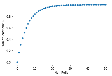
And now we are in a position to find the chance that the face with six spots comes up at least once in rolls of a die.
For example, $\(𝑃(a~single~roll~is~not~6) = 𝑃(1)+𝑃(2)+𝑃(3)+𝑃(4)+𝑃(5) = \frac{5}{6}\)$
Therefore, $\(𝑃(at~least~one~6~in~two~rolls) = 1−𝑃(both~rolls~are~not~6) = 1−(\frac{5}{6})^2\)$
and $\(𝑃(at~least~one~6~in~17~rolls) = 1−(\frac{5}{6})^{17}\)$
The table below shows these probabilities as the number of rolls increases from 1 to 50.
import pandas as pd
HowManyRollsToTake = 50
numRolls = []
probabilities = []
for i in range(HowManyRollsToTake+1):
    numRolls.append(i)
    probabilities.append(1-(5/6)**i)

rolls = {
    "NumRolls": numRolls,
    "Prob at least one 6": probabilities
}

df = pd.DataFrame(rolls)
df.plot.scatter(x="NumRolls", y="Prob at least one 6")
<AxesSubplot:xlabel='NumRolls', ylabel='Prob at least one 6'>
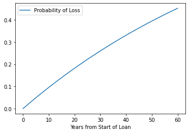
Why Should anyone buy Flood Insurance?
Lets apply these ideas to insurance.

Suppose you have a house that is located in the 100-year ARI (Annual Recurrance Interval) regulatory flood plain; and you are in a community with a good engineer, who got the probability about correct, that is the chance in any year of a total loss is 1 in 100 or 0.01. Thus the chance of no loss in any year is 99 in 100 or 0.99 (pretty good odds)!
So what is the chance during a 30-year loan, of no loss?
We can just apply the multiplication rule on the no loss probability $\( P(No~Loss) = 0.99^{30} \)$
But lets simulate - literally adapting the prior script.
import pandas as pd
HowManyYears = 60
numYears = []
nolossprobabilities = []
lossprobabilities = []
for i in range(HowManyYears+1):
    numYears.append(i) # How many years in the sequence
    nolossprobabilities.append((1-(1/100))**i) #Probability of No Loss after i-years
    lossprobabilities.append(1 - (1-(1/100))**i) #Probability of Loss after i-years
years = {
    "Years from Start of Loan": numYears,
    "Probability of No Loss": nolossprobabilities,
    "Probability of Loss": lossprobabilities
}

df = pd.DataFrame(years)
df.plot.line(x="Years from Start of Loan", y="Probability of Loss")
# df.plot.line(x="Years from Start of Loan", y="Probability of No Loss")
<AxesSubplot:xlabel='Years from Start of Loan'>
df.head(30)
| Years from Start of Loan | Probability of No Loss | Probability of Loss | |
|---|---|---|---|
| 0 | 0 | 1.000000 | 0.000000 |
| 1 | 1 | 0.990000 | 0.010000 |
| 2 | 2 | 0.980100 | 0.019900 |
| 3 | 3 | 0.970299 | 0.029701 |
| 4 | 4 | 0.960596 | 0.039404 |
| 5 | 5 | 0.950990 | 0.049010 |
| 6 | 6 | 0.941480 | 0.058520 |
| 7 | 7 | 0.932065 | 0.067935 |
| 8 | 8 | 0.922745 | 0.077255 |
| 9 | 9 | 0.913517 | 0.086483 |
| 10 | 10 | 0.904382 | 0.095618 |
| 11 | 11 | 0.895338 | 0.104662 |
| 12 | 12 | 0.886385 | 0.113615 |
| 13 | 13 | 0.877521 | 0.122479 |
| 14 | 14 | 0.868746 | 0.131254 |
| 15 | 15 | 0.860058 | 0.139942 |
| 16 | 16 | 0.851458 | 0.148542 |
| 17 | 17 | 0.842943 | 0.157057 |
| 18 | 18 | 0.834514 | 0.165486 |
| 19 | 19 | 0.826169 | 0.173831 |
| 20 | 20 | 0.817907 | 0.182093 |
| 21 | 21 | 0.809728 | 0.190272 |
| 22 | 22 | 0.801631 | 0.198369 |
| 23 | 23 | 0.793614 | 0.206386 |
| 24 | 24 | 0.785678 | 0.214322 |
| 25 | 25 | 0.777821 | 0.222179 |
| 26 | 26 | 0.770043 | 0.229957 |
| 27 | 27 | 0.762343 | 0.237657 |
| 28 | 28 | 0.754719 | 0.245281 |
| 29 | 29 | 0.747172 | 0.252828 |
df["Probability of Loss"].loc[30]
0.2602996266117198
Laboratory 18
Examine (click) Laboratory 18 as a webpage at Laboratory 18.html
Download (right-click, save target as …) Laboratory 18 as a jupyterlab notebook from Laboratory 18.ipynb
Exercise Set 18
Examine (click) Exercise Set 18 as a webpage at Exercise 18.html
Download (right-click, save target as …) Exercise Set 18 as a jupyterlab notebook at Exercise Set 18.ipynb