.ipynb .pdf

repository open issue

Binder

Contents

ENGR 1330 Computational Thinking with Data Science

Copyright © 2022 Theodore G. Cleveland and Farhang Forghanparast

Last GitHub Commit Date: Never

10: Vector/Matrix applications (Under Construction)

• curve-fitting

• linear heat flow

• network flow (Optional; Non-linear System of equations)

Linear Systems Applications

Curve-Fitting

Linear Flow of Heat

Nonlinear Systems Applications

Non-linear systems are extensions of the linear systems cases except the systems involve products and powers of the unknown variables. Non-linear problems are often quite difficult to manage, especially when the systems are large (many rows and many variables). The solution to non-linear systems, if non-trivial or even possible, are usually iterative. Within the iterative steps is a linearization component – these linear systems which are intermediate computations within the overall solution process are treated by an appropriate linear system method (direct or iterative). Consider the system below:

\( \begin{gather} \begin{matrix} x^2 & +~y^2 \\ e^x & +~y \\ \end{matrix} \begin{matrix} = 4\\ = 1\\ \end{matrix} \end{gather} \)

Suppose we have a solution guess \(x_{k},y_{k}\), which of course could be wrong, but we could linearize about that guess as

\( \begin{gather} \mathbf{A} = \begin{pmatrix} x_k & + ~y_k \\ 0 & + ~1 \\ \end{pmatrix} ~\mathbf{x} = \begin{pmatrix} x_{k+1} \\ y_{k+1} \\ \end{pmatrix} ~ \mathbf{b} = \begin{pmatrix} 4\\ 1 - e^{x_k}\\ \end{pmatrix} \end{gather} \)

Now if we assemble the system in the usual fashion, \(\mathbf{A} \cdot \mathbf{x_{k+1}} = ~ \mathbf{b}~\) we have a system of linear equations (Linear in \(\mathbf{x_{k+1}}\)}), which expanded look like:

\( \begin{gather} \begin{pmatrix} x_k & + ~y_k \\ 0 & + ~1 \\ \end{pmatrix} \cdot \begin{pmatrix} x_{k+1} \\ y_{k+1} \\ \end{pmatrix} ~ = \begin{pmatrix} 4\\ 1 - e^{x_k}\\ \end{pmatrix} \end{gather} \)

Now that the system is linear, and we can solve for \(\mathbf{x_{k+1}}\) using our linear system solver for the new guess. If the system is convergent (not all are) then if we update, and repeat we will eventually find a result.

What one really needs is a way to construct the linear system that has a systematic update method, that is discussed below

Note

The examples below use two user-defined modules listed below. Use of user-defined modules is discussed in the lesson on functions

> LinearSolverPivot.py

# SolveLinearSystem.py
# Code to read A and b
# Then solve Ax = b for x by Gaussian elimination with back substitution
#
##########
def linearsolver(A,b):
    n = len(A)
#    M = A  #this is object to object equivalence
# copy A into M element by element
    M=[[0.0 for jcol in range(n)]for irow in range(n)]
    for irow in range(n):
        for jcol in range(n):
            M[irow][jcol]=A[irow][jcol]


    i = 0
    for x in M:
     x.append(b[i])
     i += 1

    for k in range(n):
     for i in range(k,n):
       if abs(M[i][k]) > abs(M[k][k]):
          M[k], M[i] = M[i],M[k]
       else:
          pass

     for j in range(k+1,n):
         q = float(M[j][k]) / M[k][k]
         for m in range(k, n+1):
            M[j][m] -=  q * M[k][m]

    x = [0 for i in range(n)]

    x[n-1] =float(M[n-1][n])/M[n-1][n-1]
    for i in range (n-1,-1,-1):
      z = 0
      for j in range(i+1,n):
          z = z  + float(M[i][j])*x[j]
      x[i] = float(M[i][n] - z)/M[i][i]
#    print (x)
    return(x)
#

> vector_matrix_lib.py

# vector_matrix_lib.py
# useful linear algebra tools
import math   # This will import math module

def writeM(M,ir,jc,label):
    print ("------",label,"------")
    for i in range(0,ir,1):
        print (M[i][0:jc])
    print ("-----------------------------")
    #return

def writeV(V,ir,label):
    print ("------",label,"------")
    for i in range(0,ir,1):
        print (V[i])
    print ("-----------------------------")
    #return

def mmmult(amatrix,bmatrix,rowNumA,colNumA,rowNumB,colNumB):
    AB =[[0.0 for j in range(colNumB)] for i in range(rowNumA)]
    for i in range(0,rowNumA):
        for j in range(0,colNumB):
            for k in range(0,colNumA):
                AB[i][j]=AB[i][j]+amatrix[i][k]*bmatrix[k][j]
    return(AB)

def mvmult(amatrix,xvector,rowNumA,colNumA):
    bvector=[0.0 for i in range(rowNumA)]
    for i in range(0,rowNumA):
        for j in range(0,1):
            for k in range(0,colNumA):
                bvector[i]=bvector[i]+amatrix[i][k]*xvector[k]
    return(bvector)

def vvadd(avector,bvector,length):
    aplusb=[0.0 for i in range(length)]
    for i in range(length):
        aplusb[i] = avector[i] + bvector[i]
    return(aplusb)

def vvsub(avector,bvector,length):
    aminusb=[0.0 for i in range(length)]
    for i in range(length):
        aminusb[i] = avector[i] - bvector[i]
    return(aminusb)

def vdotv(avector,bvector,length):
    adotb=0.0
    for i in range(length):
        adotb=adotb+avector[i]*bvector[i]
    return(adotb)

Newton-Raphson Method

This section presents the Newton-Raphson method as a way to sometimes solve systems of non-linear equations.

Consider an example where the function \(\textbf{f}\) is a vector-valued function of a vector argument.

\( \begin{gather} \mathbf{f(x)} = \begin{matrix} f_1 = & x^2 & +~y^2 & - 4\\ f_2 = & e^x & +~y & - 1\\ \end{matrix} \end{gather} \)

Let’s also recall Newtons method for scalar valued function of a single variable.

\( \begin{equation} x_{k+1}=x_{k} - \frac{ f(x_{k}) }{ \frac{df}{dx}\rvert_{x_k} } \label{eqn:NewtonFormula} \end{equation} \)

When extending to higher dimensions, the analog for \(x\) is the vector \(\textbf{x}\) and the analog for the function \(f()\) is the vector function \(\textbf{f()}\). What remains is an analog for the first derivative in the denominator (and the concept of division of a matrix).

The analog to the first derivative is a matrix called the Jacobian which is comprised of the first derivatives of the function \(\textbf{f}\) with respect to the arguments \(\textbf{x}\).
For example for a 2-value function of 2 arguments (as our example above)

\( \begin{equation} \frac{df}{dx}\rvert_{x_k} => \begin{pmatrix} \frac{\partial f_1}{\partial x_1} & \frac{\partial f_1}{\partial x_2} \\ ~ & ~ \\ \frac{\partial f_2}{\partial x_1} & \frac{\partial f_2}{\partial x_2} \\ \end{pmatrix} \label{eqn:Jacobian} \end{equation} \)

Next recall that division is replaced by matrix multiplication with the multiplicative inverse, so the analogy continues as

\( \begin{equation} \frac{1}{\frac{df}{dx}\rvert_{x_k}} => {\begin{pmatrix} \frac{\partial f_1}{\partial x_1} & \frac{\partial f_1}{\partial x_2} \\ ~ & ~ \\ \frac{\partial f_2}{\partial x_1} & \frac{\partial f_2}{\partial x_2} \\ \end{pmatrix}}^{-1} \label{eqn:JacobianInverse} \end{equation} \)

Let’s name the Jacobian \(\textbf{J(x)}\).

So the multi-variate Newton’s method can be written as

\( \begin{equation} \mathbf{x}_{k+1}=\mathbf{x}_{k} - \mathbf{J(x)}^{-1}\rvert_{x_k} \cdot \mathbf{f(x)}\rvert_{x_k} \label{eqn:VectorNewtonFormula} \end{equation} \)

In the linear systems lessons we did find a way to solve for an inverse, but it’s not necessary, and is computationally expensive to invert in these examples – a series of rearrangement of the system above yields a nice scheme that does not require inversion of a matrix.

First, move the \(\mathbf{x}_{k}\) to the left-hand side.

\( \begin{equation} \mathbf{x}_{k+1}-\mathbf{x}_{k} = - \mathbf{J(x)}^{-1}\rvert_{x_k} \cdot \mathbf{f(x)}\rvert_{x_k} \end{equation} \)

Next multiply both sides by the Jacobian (The Jacobian must be non-singular otherwise we are dividing by zero)

\( \begin{equation} \mathbf{J(x)}\rvert_{x_k} \cdot (\mathbf{x}_{k+1}-\mathbf{x}_{k}) = - \mathbf{J(x)}\rvert_{x_k} \cdot \mathbf{J(x)}^{-1}\rvert_{x_k} \cdot \mathbf{f(x)}\rvert_{x_k} \end{equation} \)

Recall a matrix multiplied by its inverse returns the identity matrix (the matrix equivalent of unity)

\( \begin{equation} -\mathbf{J(x)}\rvert_{x_k} \cdot (\mathbf{x}_{k+1}-\mathbf{x}_{k}) = \mathbf{f(x)}\rvert_{x_k} \end{equation} \)

So we now have an algorithm:

1. Start with an initial guess \(\mathbf{x}_{k}\), compute \(\mathbf{f(x)}\rvert_{x_k}\), and \(\mathbf{J(x)}\rvert_{x_k}\).

2. Test for stopping. Is \(\mathbf{f(x)}\rvert_{x_k}\) close to zero? If yes, exit and report results, otherwise continue.

3. Solve the linear system \(\mathbf{J(x)}\rvert_{x_k} \cdot (\mathbf{x}_{k+1}-\mathbf{x}_{k}) = \mathbf{f(x)}\rvert_{x_k}\).

4. Test for stopping. Is \( (\mathbf{x}_{k+1}-\mathbf{x}_{k})\) close to zero? If yes, exit and report results, otherwise continue.

5. Compute the update \(\mathbf{x}_{k+1} = \mathbf{x}_{k} - (\mathbf{x}_{k+1}-\mathbf{x}_{k}) \), then

6. Move the update into the guess vector \(\mathbf{x}_{k} <=\mathbf{x}_{k+1}\) =and repeat step 1. Stop after too many steps.

Example using Analytical Derivatives

Now to complete the example we will employ this algorithm.

The function (repeated)

\( \begin{gather} \mathbf{f(x)} = \begin{matrix} f_1 = & x^2 & +~y^2 & - 4\\ f_2 = & e^x & +~y & - 1\\ \end{matrix} \end{gather} \)

Then the Jacobian, here we will compute it analytically because we can

\( \begin{equation} \mathbf{J(x)}=> {\begin{pmatrix} 2x & 2y \\ ~ & ~ \\ e^x & 1 \\ \end{pmatrix}} \end{equation} \)

Now for the scripts.

We will start by defining the two equations, and their derivatives, as well a a vector valued function func and its Jacobian jacob as below. Here the two modules LinearSolverPivot and vector_matrix_lib are just python source code files containing prototype functions.

#################################################################
# Newton Solver Example -- Analytical Derivatives               #
#################################################################
import math   # This will import math module from python distribution
from LinearSolverPivot import linearsolver # This will import our solver module
from vector_matrix_lib import writeM,writeV,vdotv,vvsub # This will import our vector functions

def eq1(x,y):
    eq1 = x**2 + y**2 - 4.0
    return(eq1)

def eq2(x,y):
    eq2 = math.exp(x) + y - 1.0
    return(eq2)

def ddxeq1(x,y):
    ddxeq1 = 2.0*x
    return(ddxeq1)

def ddyeq1(x,y):
    ddyeq1 = 2.0*y
    return(ddyeq1)

def ddxeq2(x,y):
    ddxeq2 = math.exp(x)
    return(ddxeq2)

def ddyeq2(x,y):
    ddyeq2 = 1.0
    return(ddyeq2)

def func(x,y):
    func  = [0.0 for i in range(2)] # null list
    # build the function
    func[0] = eq1(x,y)
    func[1] = eq2(x,y)
    return(func)

def jacob(x,y):
    jacob = [[0.0 for j in range(2)] for i in range(2)] # constructed list  
    #build the  jacobian
    jacob[0][0]=ddxeq1(x,y)
    jacob[0][1]=ddyeq1(x,y)
    jacob[1][0]=ddxeq2(x,y)
    jacob[1][1]=ddyeq2(x,y)
    return(jacob)

Next we create vectors to store values, and supply initial guesses to the system, and echo the inputs.

deltax  = [0.0 for i in range(2)] # null list
xguess  = [0.0 for i in range(2)] # null list
myfunc  = [0.0 for i in range(2)] # null list
myjacob = [[0.0 for j in range(2)] for i in range(2)] # constructed list  
# supply initial guess
xguess[0]=1.0 ; xguess[1]=0.0
#xguess[0] = float(input("Value for x : "))
#xguess[1] = float(input("Value for y : "))
# build the initial function
myfunc = func(xguess[0],xguess[1])
#build the initial jacobian
myjacob=jacob(xguess[0],xguess[1])
#write initial results
writeV(xguess,2,"Initial X vector ")
writeV(myfunc,2,"Initial FUNC vector ")
writeM(myjacob,2,2,"Initial Jacobian ")
# solver parameters
tolerancef = 1.0e-9
tolerancex = 1.0e-9

------ Initial X vector  ------
1.0
0.0
-----------------------------
------ Initial FUNC vector  ------
-3.0
1.718281828459045
-----------------------------
------ Initial Jacobian  ------
[2.0, 0.0]
[2.718281828459045, 1.0]
-----------------------------

Now we apply the algorithm a few times, here the count is set to 10. So eneter the loop, test for stopping, then update.

# Newton-Raphson
for iteration in range(10):
    myfunc = func(xguess[0],xguess[1])
    testf = vdotv(myfunc,myfunc,2)
    if testf <= tolerancef :
        print("f(x) close to zero\n test value : ", testf)
        break
    myjacob=jacob(xguess[0],xguess[1])
    deltax=linearsolver(myjacob,myfunc)
    testx = vdotv(deltax,deltax,2)
    if testx <= tolerancex :
        print("solution change small\n test value : ", testx)
        break
    xguess=vvsub(xguess,deltax,2)
##    print("iteration : ",iteration)
##    writeV(xguess,2,"Current X vector ")
##    writeV(myfunc,2,"Current FUNC vector ")
print("Exiting Iteration : ",iteration)
writeV(xguess,2,"Exiting X vector ")
writeV(myfunc,2,"Exiting FUNC vector ")

f(x) close to zero
 test value :  1.3156082836179522e-12
Exiting Iteration :  6
------ Exiting X vector  ------
1.0041690772134464
-1.7296372862705844
-----------------------------
------ Exiting FUNC vector  ------
6.776891758875081e-07
9.253894663885376e-07
-----------------------------

Quasi-Newton Method using Finite Difference Approximations for the Derivative

The next variant is to approximate the derivatives – usually a Finite-Difference approximation is used, either forward, backward, or centered differences – generally determined based on the actual behavior of the functions themselves or by trial and error.

For really huge systems, we usually make the program itself make the adaptions as it proceeds.

The coding for a finite-difference representation of a Jacobian is shown in Listing that follows In constructing the Jacobian, we observe that each column of the Jacobian is simply the directional derivative of the function with respect to the variable associated with the column.
For instance, the first column of the Jacobian in the example is first derivative of the first function (all rows) with respect to the first variable, in this case \(x\). The second column is the first derivative of the second function with respect to the second variable, \(y\).
This structure is useful to generalize the Jacobian construction method because we could write (yet another) prototype function that can take the directional derivatives for us, and just insert the returns as columns; in the example we simply modified the ddx and ddy functions from analytical to simple finite differences.

The example listing is specific to the 2X2 function in the example, but the extension to more general cases is evident.

#################################################################
# Newton Solver Example -- Numerical Derivatives               #
#################################################################
import math   # This will import math module from python distribution
from LinearSolverPivot import linearsolver # This will import our solver module
from vector_matrix_lib import writeM,writeV,vdotv,vvsub # This will import our vector functions

def eq1(x,y):
    eq1 = x**2 + y**2 - 4.0
    return(eq1)

def eq2(x,y):
    eq2 = math.exp(x) + y - 1.0
    return(eq2)
##############################################################
# This portion is changed for finite-difference method to evaluate derivatives #
##############################################################
def ddxeq1(x,y):
    delta = 1.0e-6
    ddxeq1 = (eq1(x+delta,y)-eq1(x,y))/delta
    return(ddxeq1)

def ddyeq1(x,y):
    delta = 1.0e-6
    ddyeq1 = (eq1(x,y+delta)-eq1(x,y))/delta
    return(ddyeq1)

def ddxeq2(x,y):
    delta = 1.0e-6
    ddxeq2 = (eq2(x+delta,y)-eq2(x,y))/delta
    return(ddxeq2)

def ddyeq2(x,y):
    delta = 1.0e-6
    ddyeq2 = (eq2(x,y+delta)-eq2(x,y))/delta
    return(ddyeq2)
##############################################################
def func(x,y):
    func  = [0.0 for i in range(2)] # null list
    # build the function
    func[0] = eq1(x,y)
    func[1] = eq2(x,y)
    return(func)

def jacob(x,y):
    jacob = [[0.0 for j in range(2)] for i in range(2)] # constructed list  
    #build the  jacobian
    jacob[0][0]=ddxeq1(x,y)
    jacob[0][1]=ddyeq1(x,y)
    jacob[1][0]=ddxeq2(x,y)
    jacob[1][1]=ddyeq2(x,y)
    return(jacob)
deltax  = [0.0 for i in range(2)] # null list
xguess  = [0.0 for i in range(2)] # null list
myfunc  = [0.0 for i in range(2)] # null list
myjacob = [[0.0 for j in range(2)] for i in range(2)] # constructed list  
# supply initial guess
# xguess[0] = float(input("Value for x : "))
# xguess[1] = float(input("Value for y : "))
xguess[0]=1.0 ; xguess[1]=0.0
# build the initial function
myfunc = func(xguess[0],xguess[1])
#build the initial jacobian
myjacob=jacob(xguess[0],xguess[1])
#write initial results
writeV(xguess,2,"Initial X vector ")
writeV(myfunc,2,"Initial FUNC vector ")
writeM(myjacob,2,2,"Initial Jacobian ")
# solver parameters
tolerancef = 1.0e-9
tolerancex = 1.0e-9
# Newton-Raphson
for iteration in range(10):
    myfunc = func(xguess[0],xguess[1])
    testf = vdotv(myfunc,myfunc,2)
    if testf <= tolerancef :
        print("f(x) close to zero\n test value : ", testf)
        break
    myjacob=jacob(xguess[0],xguess[1])
    deltax=linearsolver(myjacob,myfunc)
    testx = vdotv(deltax,deltax,2)
    if testx <= tolerancex :
        print("solution change small\n test value : ", testx)
        break
    xguess=vvsub(xguess,deltax,2)
##    print("iteration : ",iteration)
##    writeV(xguess,2,"Current X vector ")
##    writeV(myfunc,2,"Current FUNC vector ")
print("Exiting Iteration : ",iteration)
writeV(xguess,2,"Exiting X vector ")
writeV(myfunc,2,"Exiting FUNC vector using Finite-Differences")

------ Initial X vector  ------
1.0
0.0
-----------------------------
------ Initial FUNC vector  ------
-3.0
1.718281828459045
-----------------------------
------ Initial Jacobian  ------
[2.0000009999243673, 1.000088900582341e-06]
[2.7182831874306146, 1.000000000139778]
-----------------------------
f(x) close to zero
 test value :  1.319054848649505e-12
Exiting Iteration :  6
------ Exiting X vector  ------
1.0041690776563807
-1.7296372862709128
-----------------------------
------ Exiting FUNC vector using Finite-Differences ------
6.785798740693849e-07
9.265981886219521e-07
-----------------------------

Exercises

Write a script that forward defines the multi-variate functions and implements the Newton-Raphson technique. Implement the method, using analytical derivatives, and find a solution to:

\( \begin{gather} \begin{matrix} x^3 & +~3y^2 & = 21\\ x^2& +~2y & = -2 \\ \end{matrix} \end{gather} \)

Repeat the exercise, except use finite-differences to approximate the derivatives.

Write a script that forward defines the multi-variate functions and implements the Newton-Raphson technique. Implement the method, using analytical derivatives, and find a solution to:

\( \begin{gather} \begin{matrix} x^2 & +~ y^2 & +~z^2 & =~ 9\\ ~ & ~ & xyz & =~ 1\\ x & +~ y & -z^2 & =~ 0\\ \end{matrix} \end{gather} \)

Repeat the exercise, except use finite-differences to approximate the derivatives.

Write a script that forward defines the multi-variate functions and implements the Newton-Raphson technique. Implement the method, using analytical derivatives, and find a solution to:

\( \begin{gather} \begin{matrix} xyz & -~ x^2 & +~y^2 & =~ 1.34\\ ~ & xy &-~z^2 & =~ 0.09\\ e^x & -~ e^y & +z & =~ 0.41\\ \end{matrix} \end{gather} \)

Repeat the exercise, except use finite-differences to approximate the derivatives.

Pipeline Network Simulation

Note

The network simulator uses input files to convey the network to the program These files are listed below.

PipeNetwork.txt

4
6
200 200 200 200 200
1.00 0.67 0.67 0.67 0.67 0.5
800 800 700 700 800 600
0.00001 0.00001 0.00001 0.00001 0.00001 0.00001
0.000011
1 1 1 1 1 1
1 -1 0 -1 0 0
0 1 -1 0 0 1
0 0 0 1 -1 -1
0 0 1 0 1 0
0 4 3 1 -100 0 0 0 0 0 

Background: Pipelines and Networks

Pipe networks are analyzed for head losses in order to size pumps, determine demand management strategies, and precict minimum pressures in the system.

Pipe Networks – Topology

Network topology refers to the layout and connections.
Networks are built of nodes (junctions) and arcs (links).

Continunity (at a node)

Water is considered incompressible in steady flow in pipelines and pipe networks, and the conservation of mass reduces to the volumetric flow rate, \(Q\),

\(Q = AV\)

where \(A\) is the cross sectional of the pipe, and \(V\) is the mean section velocity. Typical units for discharge is liters per second (lps), gallons per minute (gpm), cubic meters per second (cms), cubic feet per second (cfs), and million gallons per day (mgd).

The continuity equation in two cross-sections of a pipe as depicted in Fig. 8 is

\( A_1V_1 = A_2V_2 \)

Junctions (nodes) are where two or more pipes join together. A three-pipe junction node with constant external demand is shown in Fig. 9.

The continuity equation for the junction node is \begin{equation} Q_1 - Q_2 - Q_3 - D = 0 \end{equation}

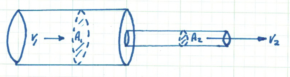
Fig. 8 Continuity of mass (discharge) across a change in cross section

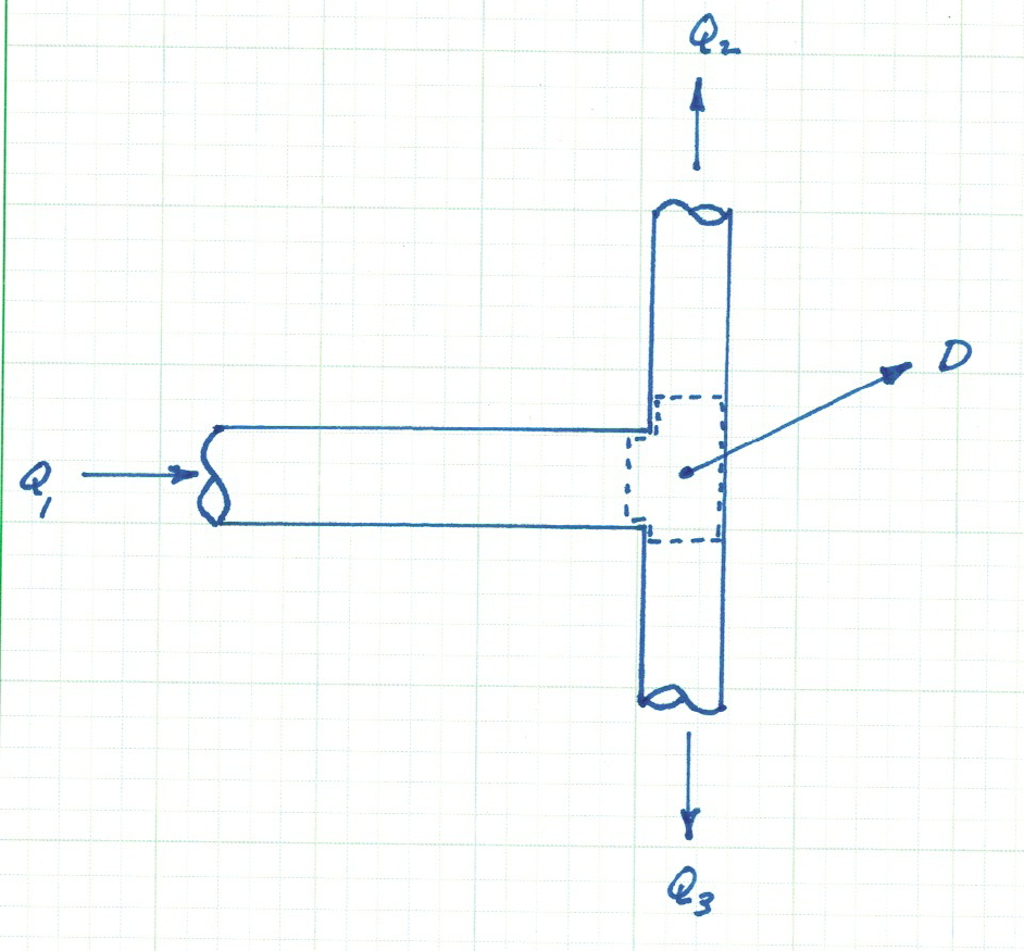
Fig. 9 Continuity of mass (discharge) across a node (junction)

In pipe network analysis, all demands on the system are stipulated to belocated at junctions (nodes), and the flow connecting junctions is assumed to be uniform across the cross sections (so that mean velocities apply). If a substantial demand is located between nodes, then an additional node is established at the demand location.

Energy Loss (along a link)

The equation below is the one-dimensional steady flow form of the energy equation typically applied for pressurized conduit hydraulics.

\( \begin{equation} \frac{p_1}{\rho g}+\alpha_1 \frac{V_1^2}{2g} + z_1 + h_p = \frac{p_2}{\rho g}+\alpha_2 \frac{V_2^2}{2g} + z_2 + h_t + h_l \label{eqn:closed-conduit-energy-equation} \end{equation} \)

where \(\frac{p}{\rho g}\) is the pressure head at a location, \(\alpha \frac{V^2}{2g}\) is the velocity head at a location, \(z\) is the elevation, \(h_p\) is the added head from a pump, \(h_t\) is the added head extracted by a turbine, and \(h_l\) is the head loss between sections 1 and 2. Fig. 10 is a sketch that illustrates the various components in the energy equation.

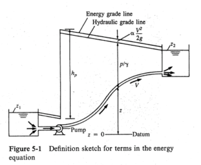
Fig. 10 Definition sketch for energy equation

In network analysis this energy equation is applied to a link that joins two nodes. Pumps and turbines would be treated as separate components (links) and their hydraulic behavior must be supplied using their respective pump/turbine curves.

Velocity Head

The velocity in \(\alpha \frac{V^2}{2g}\) is the mean section velocity and is the ratio of discharge to flow area. The kinetic energy correction coefficient is \(\begin{equation} \alpha=\frac{\int_A u^3 dA}{V^3 A} \label{eqn:kinetic-energy-correction} \end{equation} \) where \(u\) is the point velocity in the cross section (usually measured relative to the centerline or the pipe wall; axial symmetry is assumed). Generally values of \(\alpha\) are 2.0 if the flow is laminar, and approach unity (1.0) for turbulent flow. In most water distribution systems the flow is usually turbulent so \(\alpha\) is assumed to be unity and the velocity head is simply \(\frac{V^2}{2g}\).

Added Head — Pumps

The head supplied by a pump is related to the mechanical power supplied to the flow. Equation \ref{eqn:pump-power} is the relationship of mechanical power to added pump head. \( \begin{equation} \eta P=Q\rho g h_p \label{eqn:pump-power} \end{equation} \) where the power supplied to the motor is \(P\) and the “wire-to-water” efficiency is \(\eta\).

If the relationship is re-written in terms of added head(A negative head loss!} the pump curve is \( \begin{equation} h_p = \frac{\eta P}{Q\rho g} \label{eqn:pump-curve} \end{equation} \)

This relationship illustrates that as discharge increases (for a fixed power) the added head decreases. Power scales at about the cube of discharge, so pump curves for computational application typically have a mathematical structure like \( \begin{equation} h_p = H_{\text{shutoff}} - K_{\text{pump}}Q^{\text{exponent}} \label{eqn:pump-curve-2} \end{equation} \)

Extracted Head — Turbines

The head recovered by a turbine is also an “added head” but appears on the loss side of the equation.
The power that can be recovered by a turbine (again using the concept of “water-to-wire” efficiency is \( \begin{equation} P=\eta Q\rho g h_t \label{eqn:turbine-power} \end{equation} \)

Pipe Head Loss Models

The Darcy-Weisbach, Chezy-Manning, and Hazen-Williams formulas are relationships between physical pipe characteristics, flow parameters, and head loss. The Darcy-Weisbach formula is the most consistent with the energy equation formulation being derivable (in structural form) from elementary principles (continunity and linear momentum), whereas the other two are empirical (despite the empirical nature of these two models all three are of practical use, and given a choice select your favorite!)

\( \begin{equation} h_{L_f}=f \frac{L}{D} \frac{V^2}{2g} \label{eqn:dw-headloss} \end{equation} \)

where \(h_{L_f}\) is the head loss from pipe friction, \(f\) is a dimensionless friction factor, \(L\) is the pipe length, \(D\) is the pipe characteristic diameter, \(V\) is the mean section velocity, and \(g\) is the gravitational acceleration.

The friction factor, \(f\), is a function of Reynolds number \(Re_D\) and the roughness ratio \(\frac{k_s}{D}\). \( \begin{equation} f=\sigma(Re_D,\frac{k_s}{D}) \label{eqn:friction-factor-dimensionless} \end{equation} \)

The structure of \(\sigma\) is determined experimentally. Over the last century the structure is generally accepted to be one of the following depending on flow conditions and pipe properties

Laminar flow (Eqn 2.36, pg. 17~\cite{chin2006}) :

\(\begin{equation} f=\frac{64}{Re_D} \label{eqn:friction-factor-laminar} \end{equation} \)

Hydraulically Smooth Pipes(Eqn 2.34 pg. 16~\cite{chin2006}):

\(\begin{equation} \frac{1}{\sqrt{f}}=-2 log_{10} (\frac{2.51}{Re_d \sqrt{f} }) \label{eqn:friction-factor-smooth} \end{equation} \)

Hydraulically Rough Pipes(Eqn 2.34 pg. 16~\cite{chin2006}):

\( \begin{equation} \frac{1}{\sqrt{f}}=-2 log_{10} (\frac{\frac{k_e}{D}} {3.7}) \label{eqn:friction-factor-rough} \end{equation} \)

Transitional Pipes (Colebrook-White Formula)(Eqn 2.35 pg. 17~\cite{chin2006}):

\( \begin{equation} \frac{1}{\sqrt{f}}=-2 log_{10} (\frac{\frac{k_e}{D}} {3.7} + \frac{2.51}{Re_d \sqrt{f} } ) \label{eqn:friction-factor-CW} \end{equation} \)

Transitional Pipes (Jain Formula)(Eqn 2.39 pg. 19~\cite{chin2006}):

\(\begin{equation} f=\frac{0.25}{[log_{10} (\frac{\frac{k_e}{D}} {3.7} + \frac{5.74}{Re_d^{0.9} } )] ^2} \label{eqn:friction-factor-Jain} \end{equation} \)

Pipe Networks Solution Methods

Several methods are used to produce solutions (estimates of discharge, head loss, and pressure) in a network.
An early one, that only involves analysis of loops is the Hardy-Cross method.
A later one, more efficient, is a Newton-Raphson method that uses node equations to balance discharges and demands, and loop equations to balance head losses.

However, a rather ingenious method exists developed by \cite{Haman1971}, where the flow distribution and head values are determined simultaneously. The task here is to outline the \cite{Haman1971} method on the problem below – first some necessary definitions and analysis.

The fundamental procedure is:

• Continuity is written at nodes (node equations).

• Energy loss (gain) is written along links (pipe equations).

• The entire set of equations is solved simultaneously.

Network Analysis Example

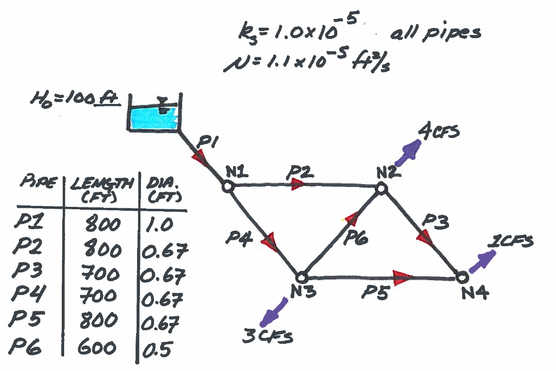
Fig. 11 Pipe network for illustrative example with supply and demands identified. Pipe dimensions and diameters are also depicted.

Fig. 11 is a sketch of the problem that will be used.
The network supply is the fixed-grade node in the upper left hand corner of the drawing.
The remaining nodes (N1 – N4) have demands specified as the purple outflow arrows. The pipes are labeled (P1 – P6), and the red arrows indicate a positive flow direction, that is, if the flow is in the indicated direction, the numerical value of flow (or velocity) in that link would be a positive number.

Define the flows in each pipe and the total head at each node as \(Q_i\) and \(H_i\) where the subscript indicates the particular component identification. Expressed as a vector, these unknowns are:

\( \begin{matrix} [Q_1, & Q_2, & Q_3, & Q_4, & Q_5, & Q_6, & H_1, & H_2, & H_3, &H_4 ]& = & \textbf{x} \\ \end{matrix} \)

If we analyze continuity for each node we will have 4 equations (corresponding to each node) for continunity, for instance for Node N2 the equation is

\( \begin{matrix} ~& Q_2 & -Q_3 & ~ & ~ & Q_6 & ~ & ~ & ~ &~ & = & 4\\ \end{matrix} \)

Similarily if we define head loss in any pipe as \(\Delta H_i = f \frac{8 L_i}{\pi^2 g D_i^5} |Q_i| Q_i\) or \(\Delta H_i = L_i Q_i\), where \(L_i = f \frac{8 L_i}{\pi^2 g D_i^5} |Q_i|\), then we have 6 equations (corresponding to each pipe) for energy, for instance for Pipe (P2) the equation is:

\( \begin{matrix} ~& -L_2Q_2& ~ & ~ & ~ & ~& H_1 & -H_2 & ~ & ~ & = & 0\\ \end{matrix} \)

If we now write all the node equations then all the pipe equations we could construct the following coefficient matrix below

Note

The horizontal lines divide the node and the pipe equations.

The upper partition are the node equations in Q and H, the lower partition are the pipe equations in Q and H}

\( \begin{matrix} \hline ~1&-1 & 0 & -1 & 0 & 0 & 0 & 0 & 0 &0 \\ 0&~1 & -1 & 0 & 0 &~1 & 0 & 0 & 0 &0 \\ 0& 0 & 0 &~1 & -1 & -1 & 0 & 0 & 0 &0 \\ 0& 0 &~1 & 0 &~1 & 0 & 0 & 0 & 0 &0 \\ \hline -L_1& 0& 0 & 0 & 0 & 0 & -1 & 0 & 0 &0 \\ 0& -L_2& 0 & 0 & 0 & 0&~1 & -1 & 0 &0 \\ 0& 0& -L_3 & 0 & 0 & 0& 0 &~1 & 0 & -1 \\ 0& 0& 0 & -L_4 & 0 & 0&~1 & 0 & -1 & 0 \\ 0& 0& 0 & 0 & -L_5 & 0& 0 & 0 &~1 & -1 \\ 0& 0& 0 &0 & 0 & -L_6& 0 & -1 &~1 & 0 \\ \hline \end{matrix} \)

Declare the name of this matrix \(\textbf{A(x)}\), where \(\textbf{x}\) denotes the unknown vector of Q augmented by H as above. Next consider the right-hand-side at the correct solution (as of yet still unknown!) as

\( \begin{matrix} [0, & 4, & 3, & 1, & -100 , & 0, & 0, & 0, & 0, &0 ] = \textbf{b}\\ \end{matrix} \)

So if the coefficient matrix is correct then the following system would result: \( \mathbf{A(x)} \cdot \mathbf{x} = \mathbf{b} \)

which would look like

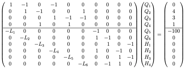
Fig. 12 Pipe network illustrative example as Matrtx-Vector system of equations.

Observe, the system is non-linear because the coefficient matrix depends on the current values of \(Q_i\) for the \(L_i\) terms. However, the system is full-rank (rows == columns) so it is a candidate for Newton-Raphson.

Further observe that the upper partition from column 6 and smaller is simply the node-arc incidence matrix, and the lower partition for the same columns only contains \(L_i\) terms on its diagonal, the remainder is zero.
Next observe that the partition associated with heads in the node equations is the zero-matrix.

Lastly (and this is important!) the lower right partition is the transpose of the node-arc incidence matrix subjected to scalar multiplication of \(-1\). The importance is that all the information needed to find a solution is contained in the node-arc incidence matrix and the right-hand-side – the engineer does not need to identify closed loops (nor does the computer need to find closed loops).

The trade-off is a much larger system of equations, however solving large systems is far easier that searching a directed graph to identify closed loops, furthermore we obtain the heads as part of the solution process.

Script Structure

The script will need to accomplish several tasks including reading the node-arc incidence matrix supplied as a file and convert the strings into numeric values. The script will also need some support functions defined before constructing the matrix. First the file for the example is:

PipeNetwork.txt

4
6
200.0 200.0 200.0 200.0 
1.00 0.67 0.67 0.67 0.67 0.5
800 800 700 700 800 600
0.00001 0.00001 0.00001 0.00001 0.00001 0.00001
0.000011
1 1 1 1 1 1
1 -1 0 -1 0 0
0 1 -1 0 0 1
0 0 0 1 -1 -1
0 0 1 0 1 0
0 4 3 1 -000 0 0 0 0 0 

The rows of the input file are:

• The node count.

• The pipe count.

• Pipe diameters, in feet.

• Pipe lengths, in feet.

• Pipe roughness heights, in feet.

• Kinematic viscosity in feet\(^2\)/second.

• Initial guess of flow rates (unbalanced OK, non-zero vital!)

• The next four rows are the node-arc incidence matrix.

• The last row is the demand (and fixed-grade node total head) vector.

Support Functions

The Reynolds number will need to be calculated for each pipe at each iteration of the solution, so a Reynolds number function will be useful. For circular pipes, the following equation should work,

\(Re_D=\frac{V_i \cdot D_i }{\mu}\)

The Jain equation (Jain, 1976) that directly computes friction factor from Reynolds number, diameter, and roughness is

\(f= \frac{0.25}{(log_{10}(\frac{\epsilon}{3.7D}+\frac{5.74}{Re_D^{0.9}}))^2}\)

Once you have the Reynolds number for a pipe, and the friction factor, then the head loss factor that will be used in the coefficient matrix (and the Jacobian) is

\(k_i = \frac{8 \cdot L_i}{\pi^2 g D_i^5}\)

We will also find it handy to be able to compute velocity heads from discharge and pipe diameters so we can have a velocity function as

\(V_i = \frac{Q_i}{0.25 \cdot \pi D_i^2}\)

These support functions are coded below (in a code cell) as:

# hydraulic elements prototype functions
# Jain Friction Factor Function -- Tested OK 23SEP16
import math   # This will import math module

def friction_factor(roughness,diameter,reynolds):
    temp1 = roughness/(3.7*diameter)
    temp2 = 5.74/(reynolds**(0.9))
    temp3 = math.log10(temp1+temp2)
    temp3 = temp3**2
    friction_factor = 0.25/temp3
    return(friction_factor)

# Velocity Function
def velocity(diameter,discharge):
    velocity=discharge/(0.25*math.pi*diameter**2)
    return(velocity)

# Reynolds Number Function  
def reynolds_number(velocity,diameter,mu):
    reynolds_number = abs(velocity)*diameter/mu
    return(reynolds_number)

# Geometric factor function
def k_factor(howlong,diameter,gravity):
    k_factor = (16*howlong)/(2.0*gravity*math.pi**2*diameter**5)
    return(k_factor)

We will need our linear solver:

# SolveLinearSystem.py
# Code to read A and b
# Then solve Ax = b for x by Gaussian elimination with back substitution
#
##########
def linearsolver(A,b):
    n = len(A)
#    M = A  #this is object to object equivalence
# copy A into M element by element - to operate on M without destroying A
    M=[[0.0 for jcol in range(n)]for irow in range(n)]
    for irow in range(n):
        for jcol in range(n):
            M[irow][jcol]=A[irow][jcol]

#
    i = 0
    for x in M:
     x.append(b[i])
     i += 1

    for k in range(n):
     for i in range(k,n):
       if abs(M[i][k]) > abs(M[k][k]):
          M[k], M[i] = M[i],M[k]
       else:
          pass

     for j in range(k+1,n):
         q = float(M[j][k]) / M[k][k]
         for m in range(k, n+1):
            M[j][m] -=  q * M[k][m]

    x = [0 for i in range(n)]

    x[n-1] =float(M[n-1][n])/M[n-1][n-1]
    for i in range (n-1,-1,-1):
      z = 0
      for j in range(i+1,n):
          z = z  + float(M[i][j])*x[j]
      x[i] = float(M[i][n] - z)/M[i][i]
#    print (x)
    return(x)
#

We will also find some vector-matrix manipulation functions handy

def writeM(M,ir,jc,label):
    print ("------",label,"------")
    for i in range(0,ir,1):
        print (M[i][0:jc])
    print ("-----------------------------")
    return()

def writeV(V,ir,label):
    print ("------",label,"------")
    for i in range(0,ir,1):
        print (V[i])
    print ("-----------------------------")
    return()

def matrixmatrixmult(amatrix,bmatrix,rowNumA,colNumA,rowNumB,colNumB):
    AB =[[0.0 for j in range(colNumB)] for i in range(rowNumA)]
    for i in range(0,rowNumA):
        for j in range(0,colNumB):
            for k in range(0,colNumA):
                AB[i][j]=AB[i][j]+amatrix[i][k]*bmatrix[k][j]
    return(AB)

def matrixvectormult(amatrix,xvector,rowNumA,colNumA):
    bvector=[0.0 for i in range(rowNumA)]
    for i in range(0,rowNumA):
        for j in range(0,1):
            for k in range(0,colNumA):
                bvector[i]=bvector[i]+amatrix[i][k]*xvector[k]
    return(bvector)

def vectoradd(avector,bvector,length):
    cvector=[]
    for i in range(length):
        cvector.append(avector[i]+bvector[i])
    return(cvector)

def vectorsub(avector,bvector,length):
    cvector=[]
    for i in range(length):
        cvector.append(avector[i]-bvector[i])
    return(cvector)
             
def vdotv(avector,bvector,length):
    adotb=0.0
    for i in range(length):
        adotb=adotb+avector[i]*bvector[i]
    return(adotb)

Augmented and Jacobian Matrices

The \(\textbf{A(x)}\) is built using the node-arc incidence matrix (which does not change), and the current values of \(L_i\).
We also need to build the Jacobian of \(\textbf{A(x)}\) to implement the update as-per Newton-Raphson.

A brief review; at the solution we can write \(\begin{equation} [\mathbf{A}(\mathbf{x})] \cdot \mathbf{x} - \mathbf{b} = \mathbf{f}(\mathbf{x}) = \mathbf{0} \end{equation} \)

Lets assume we are not at the solution, so we need a way to update the current value of \(\textbf{x}\). Recall from Newton’s method (for univariate cases) that the update formula is

\( \begin{equation} x_{k+1}=x_{k} - (\frac{df}{dx}\mid_{x_k})^{-1} f(x_k) \end{equation} \)

The Jacobian will play the role of the derivative, and \(\textbf{x}\) is now a vector (instead of a single variable). Division is not defined for matrices, but the multiplicative inverse is (the inverse matrix), and plays the role of division. Hence, the extension to the pipeline case is

\( \begin{equation} \mathbf{x}_{k+1}=\mathbf{x}_{k} - [\mathbf{J}(\mathbf{x}_{k})]^{-1} \mathbf{f}(\mathbf{x}_k) \end{equation} \)

where \(\mathbf{J}(\mathbf{x}_{k})\) is the Jacobian of the coefficient matrix \(\mathbf{A}\) evaluated at \(\mathbf{x}_{k}\).
Although a bit cluttered, here is the formula for a single update step, with the matrix, demand vector, and the solution vector in their proper places.

\( \begin{equation} \mathbf{x}_{k+1}=\mathbf{x}_{k} - [\mathbf{J}(\mathbf{x}_{k})]^{-1} \{[\mathbf{A}(\mathbf{x}_k)] \cdot \mathbf{x}_k - \mathbf{b}\} \end{equation} \)

As a practical matter we actually never invert the Jacobian, instead we solve the related Linear system of

\( [\mathbf{J}(\mathbf{x}_{k})] \cdot \Delta \mathbf{x} = \{[\mathbf{A}(\mathbf{x}_k)] \cdot \mathbf{x}_k - \mathbf{b}\} \)

for \(\Delta\textbf{x}\), then perform the update as \(\textbf{x}_{k+1} = \textbf{x}_{k} - \Delta\textbf{x}\)

Note

Inverting the matrix every step is computationally inefficient, and unnecessary. As an example, solving the system in this case would at worst take 10 row operations each step, but nearly 100 row operations to invert at each step – to accomplish the same result, generate an update. Now imagine when there are hundreds of nodes and pipes!

The Jacobian of the pipeline model is a matrix with the following properties:

• The partition of the matrix that corresponds to the node formulas (upper left partition) is identical to the original coefficient matrix — it will be comprised of \(0~\text{or}~\pm~1\) in the same pattern at the equivalent partition of the \(\mathbf{A}\) matrix.

• The partition of the matrix that corresponds to the pipe head loss terms (lower left partition), will consist of values that are twice the values of the coefficients in the original coefficient matrix (at any supplied value of \(\mathbf{x}_k\).

• The partition of the matrix that corresponds to the head terms (lower right partition), will consist of values that are identical to the original matrix.

• The partition of the matrix that corresponds to the head coefficients in the node equations (upper right partition) will also remain unchanged.

We will want to take advantage of problem structure to build the Jacobian (you could just finite-difference the coefficient matrix to approximate the partial derivatives, but that is terribly inefficient if you already know the structure).

So now lets code reading the input file and building at least the starting instance of the matrix equations

First allocate some memory

bvector = []
rowNumA = 0
colNumA = 0
rowNumB = 0
verbose = 'false' # set to true for in-class demonstration
#############################################

elevation = [] # null list node elevations
diameter =  [] # null list pipe diameters
distance =  [] # null list pipe lengths
roughness = [] # null list pipe roughness
flowguess = [] # null list pipe flow rates
nodearcs =  [] # node-arc incidence matrix
rhs_true =  [] # null list for nodal demands
tempvect = []

Now read in the data from a file (useful to expand problem scale to many,many pipes and nodes).

##############################################
# connect and read file for Pipeline Network #
##############################################
afile = open("PipeNetwork.txt","r")
nnodes = int(afile.readline())
npipes = int(afile.readline())
# read elevation vector
tempvect.append([float(n) for n in afile.readline().strip().split()])
for i in range(0,nnodes,1):
    elevation.append(float(tempvect[0][i]))
tempvect = [] # reset vector
# read diameter vector
tempvect.append([float(n) for n in afile.readline().strip().split()])
for i in range(0,npipes,1):
    diameter.append(float(tempvect[0][i]))
tempvect = [] # reset vector
# read length vector
tempvect.append([float(n) for n in afile.readline().strip().split()])
for i in range(0,npipes,1):
    distance.append(float(tempvect[0][i]))
tempvect = [] # reset vector
# read roughness vector
tempvect.append([float(n) for n in afile.readline().strip().split()])
for i in range(0,npipes,1):
    roughness.append(float(tempvect[0][i]))
tempvect = [] # reset vector
# read viscosity (scalar)
viscosity = float(afile.readline())
# read current flow guess
tempvect.append([float(n) for n in afile.readline().strip().split()])
for i in range(0,npipes,1):
    flowguess.append(float(tempvect[0][i]))
tempvect = [] # reset vector
# read nodearc incidence matrix
## future revisions read directly into augmented matrix, or find way to release nodearc from stack
for irow in range(0,nnodes,1):  # then read each row
    nodearcs.append([float(n) for n in afile.readline().strip().split()])
# read demands guess
tempvect.append([float(n) for n in afile.readline().strip().split()])
for i in range(0,nnodes+npipes,1):
    rhs_true.append(float(tempvect[0][i]))
tempvect = [] # reset vector      
######################################
# end file read ,disconnect file     #
######################################
afile.close() # Disconnect the file

Echo the data just read, could put into a conditional and choose not to display except for debugging.

######################################
# echo the input in human readable   #
######################################
print('number of nodes : ',nnodes)
print('number of pipes : ',npipes)
print('viscosity       : ',viscosity)
print ("-----------------------------")
for irow in range(0,nnodes):
    print('node id:',irow, ', elevation :',elevation[irow],' head :',rhs_true[irow+npipes])
print ("-----------------------------")
for jcol in range(0,npipes):
    print('pipe id:',jcol,', diameter : ' ,diameter[jcol],', distance : ',distance[jcol],
          ', roughness : ',roughness[jcol],', flow  : ',flowguess[jcol])
print ("-----------------------------")
##for jcol in range(0,nnodes+npipes):
##    print('irow :',jcol,' RHS True :',rhs_true[jcol])
##print ("-----------------------------")
print("node-arc incidence matrix")
for i in range(0,nnodes,1):
    print (nodearcs[i][0:npipes])
print ("-----------------------------")

number of nodes :  4
number of pipes :  6
viscosity       :  1.1e-05
-----------------------------
node id: 0 , elevation : 0.0  head : 0.0
node id: 1 , elevation : 0.0  head : 0.0
node id: 2 , elevation : 0.0  head : 0.0
node id: 3 , elevation : 0.0  head : 0.0
-----------------------------
pipe id: 0 , diameter :  1.0 , distance :  800.0 , roughness :  1e-05 , flow  :  1.0
pipe id: 1 , diameter :  0.67 , distance :  800.0 , roughness :  1e-05 , flow  :  1.0
pipe id: 2 , diameter :  0.67 , distance :  700.0 , roughness :  1e-05 , flow  :  1.0
pipe id: 3 , diameter :  0.67 , distance :  700.0 , roughness :  1e-05 , flow  :  1.0
pipe id: 4 , diameter :  0.67 , distance :  800.0 , roughness :  1e-05 , flow  :  1.0
pipe id: 5 , diameter :  0.5 , distance :  

600.0 , roughness :  1e-05 , flow  :  1.0
-----------------------------
node-arc incidence matrix
[1.0, -1.0, 0.0, -1.0, 0.0, 0.0]
[0.0, 1.0, -1.0, 0.0, 0.0, 1.0]
[0.0, 0.0, 0.0, 1.0, -1.0, -1.0]
[0.0, 0.0, 1.0, 0.0, 1.0, 0.0]
-----------------------------

Now create the augmented matrix using the structure of the problem.

# create augmented matrix
colNumA = npipes+nnodes
rowNumA = nnodes+npipes
augmentedMat = [] # null list to store augmented matrix

#######################################################################################
augmentedMat = [[0.0 for j in range(colNumA)]for i in range(rowNumA)] #fill with zeroes
#build upper left partition -- from nodearcs
for ir in range(0,nnodes):
    for jc in range (0,npipes):
        augmentedMat[ir][jc] = nodearcs[ir][jc]
istart=nnodes
iend=nnodes+npipes
jstart=npipes
jend=npipes+nnodes
for ir in range(istart,iend):
    for jc in range (jstart,jend):
        augmentedMat[ir][jc] = -1.0*nodearcs[jc-jstart][ir-istart] + 0.0
if verbose == 'true' :
    print("augmented matrix before loss factors")
    writeM(augmentedMat,rowNumA,colNumA,"augmented matrix")

Stopping Criteria, and Solution Report}

You will need some way to stop the process – the three most obvious (borrowed from Newton’s method) are:

• Approaching the correct solution (e.g. \([\mathbf{A}(\mathbf{x})] \cdot \mathbf{x} - \mathbf{b} = \mathbf{f}(\mathbf{x}) = \mathbf{0}\)).

• Update vector is not changing (e.g. \(\mathbf{x}_{k+1}=\mathbf{x}_{k}\)), so either have an answer, or the algorithm is stuck.

• You have done a lot of iterations (say 100).

We want to have the script determine when to stop and report the conditions (which stopping criterion was used), and the values of flows and heads in the system.

Fisrt lets set some tolerances and an iteration limit, as well as allocate memory to store the auxiliary functions results

#######################################################################################
howmany=50 #iterations max
tolerance1 = 1e-24
tolerance2 = 1e-24
velocity_pipe = [0 for i in range(npipes)]  # null list velocities
reynolds      = [0 for i in range(npipes)]  # null list reynolds numbers
friction      = [0 for i in range(npipes)]  # null list friction 
geometry      = [0 for i in range(npipes)]  # null list geometry
lossfactor    = [0 for i in range(npipes)]  # null list loss
jacbMat = [] # null list to store jacobian matrix
jacbMat = [[0.0 for j in range(colNumA)]for i in range(rowNumA)] #fill with zeroes


solvecguess =[ 0.0 for i in range(rowNumA)] 
solvecnew =[ 0.0 for i in range(rowNumA)]
for i in range(0,npipes,1):
    solvecguess[i] = flowguess[i]
    geometry[i] = k_factor(distance[i],diameter[i],32.2)
#solvecguess is a current guess -- wonder if more pythonic way for this assignment
##    print('irow :',i,' Geometry Factor :',geometry[i])
##print ("-----------------------------")

And finally the money shot; where we wrap everything into a for loop to iteratively find a solution

###############################################################
## ITERATION LOOP                                             #
###############################################################
for iteration in range(howmany): # iteration outer loop
    if verbose == 'true' :
        print("solutions at begin of iteration",iteration)
        for jcol in range(0,nnodes+npipes):
            print('irow :',jcol,' solvecnew :',solvecnew[jcol]," solvecguess ",solvecguess[jcol])
        print ("-----------------------------")
    for i in range(0,npipes,1):
        velocity_pipe[i] = velocity(diameter[i],flowguess[i])    
        reynolds[i]=reynolds_number(velocity_pipe[i],diameter[i],viscosity)
        friction[i]=friction_factor(roughness[i],diameter[i],reynolds[i])
        lossfactor[i]=friction[i]*geometry[i]*abs(flowguess[i])
    if verbose == 'true' :
        for jcol in range(0,npipes):
            print('pipe id:',jcol,', velocity : ' ,velocity_pipe[jcol],', reynolds : ',reynolds[jcol],
          ', friction : ',friction[jcol],', loss factor : ',lossfactor[jcol],'flow guess',flowguess[jcol])
################################################################
# BUILD AUGMENTED MATRIX CURRENT Q+H SOLUTION                  #
################################################################
    augmentedMat = [[0.0 for j in range(colNumA)]for i in range(rowNumA)] #fill with zeroes
    #build upper left partition -- from nodearcs
    for ir in range(0,nnodes):
        for jc in range (0,npipes):
            augmentedMat[ir][jc] = nodearcs[ir][jc]
    #build lower right == transpose of upper left
    istart=nnodes
    iend=nnodes+npipes
    jstart=npipes
    jend=npipes+nnodes
    for ir in range(istart,iend):
        for jc in range (jstart,jend):
            augmentedMat[ir][jc] = -1.0*nodearcs[jc-jstart][ir-istart] + 0.0
    # build lower left partition of the matrix
    istart = nnodes
    iend = nnodes+npipes
    jstart = 0
    jend = npipes
    for i in range(istart,iend ):
        for j in range(jstart,jend ):
    #        print('i =',i,'j=',j)
            if (i-istart) == j :
    #            print('i =',i,'j=',j)
                augmentedMat[i][j] = -1.0*lossfactor[j] + 0.0
    if verbose == 'true' :
        print("updated augmented matrix in iteration",iteration)
        writeM(augmentedMat,rowNumA,colNumA,"augmented matrix")
################################################################
# BUILD JACOBIAN MATRIX CURRENT Q+H SOLUTION                   #
################################################################        
    # now build current jacobian
    for i in range(rowNumA):
        for j in range(colNumA):
            jacbMat[i][j] = augmentedMat[i][j]
    # modify lower left partition
    istart = nnodes
    iend = nnodes+npipes
    jstart = 0
    jend = npipes
    for i in range(istart,iend ):
        for j in range(jstart,jend ):
    #        print('i =',i,'j=',j)
            if (i-istart) == j :
    #            print('i =',i,'j=',j)
                jacbMat[i][j] = 2.0*jacbMat[i][j]
##        for jcol in range(0,nnodes+npipes):
##            print('irow :',jcol,' solvecnew :',solvecnew[jcol]," solvecguess ",solvecguess[jcol])
##        print ("-----------------------------")
# matrix multiply augmentedMat*solvecguess to get current g(Q)
#    gq = [0.0 for i in range(rowNumA)] # zero gradient vector
##    if verbose == 'true' :
##        print("augmented matrix in iteration",iteration)
##        writeM(augmentedMat,rowNumA,colNumA,"augmented matrix before mmult")
    gq = matrixvectormult(augmentedMat,solvecguess,rowNumA,colNumA)
##    if verbose == 'true' :
##        writeV(gq,rowNumA,"gq vectorbefore subtract rhs_true")
# subtract rhs
#    for i in range(rowNumA):
    gq = vectorsub(gq,rhs_true,rowNumA)#vector subtract
    if verbose == 'true' :
        print("computed g(q) in iteration",iteration)
        writeV(gq,rowNumA,"gq vector")
        print("compare current and new guess")
        for jcol in range(0,nnodes+npipes):
            print('irow :',jcol,' solvecnew :',solvecnew[jcol]," solvecguess ",solvecguess[jcol])
        print ("-----------------------------")
    dq = [0.0 for i in range(rowNumA)] # zero update vector
    if verbose == 'true' :
        writeV(dq,rowNumA,"dq vector before linear solve")
    if verbose == 'true' :
        print("jacobian before linearsolve in iteration",iteration)
        writeM(jacbMat,rowNumA,colNumA,"jabobian matrix")
    dq = linearsolver(jacbMat,gq) # memory leak after this call - linearsolve clobbers input lists
#    dq = np.linalg.solve(jacbMat,gq)
    if verbose == 'true' :
        print("jacobian after linearsolve in iteration",iteration)
        writeM(jacbMat,rowNumA,colNumA,"jabobian matrix")

    if verbose == 'true' :
        writeV(dq,rowNumA,"dq vector -after linear solve")
    solvecnew = vectorsub(solvecguess,dq,rowNumA)#vector subtract
    if verbose == 'true' :
        print("Q_new = Q_old - DQ")
        writeV(solvecnew,rowNumA,"new guess vector")
#    tempvect =[ 0.0 for i in range(rowNumA)]
##        tempvect = matrixvectormult(jacbMat,dq,rowNumA,colNumA)
##        writeV(tempvect,rowNumA,"J*dq vector")
##        tempvect = vectorsub(tempvect,gq,rowNumA)
##        writeV(tempvect,rowNumA,"J*dq - gq vector")
        print("just after computing new guess, should be different")
        for jcol in range(0,nnodes+npipes):
            print('irow :',jcol,' solvecnew :',solvecnew[jcol]," solvecguess ",solvecguess[jcol])
        print ("-----------------------------")
#test for stopping
    tempvect =[ 0.0 for i in range(rowNumA)]
    for i in range(rowNumA):
        tempvect[i] = abs(solvecnew[i] - solvecguess[i])
    test1 = vdotv(tempvect,tempvect,rowNumA)
    if verbose == 'true' :
        print('test1',test1)
    tempvect =[ 0.0 for i in range(rowNumA)]
    for i in range(rowNumA):
        tempvect[i] = abs(gq[i])
    test2 = vdotv(tempvect,tempvect,rowNumA)
    if verbose == 'true' :
        print('test2',test2)
    if test1 < tolerance1 :
        print("update not changing --exit and report current update")
        print("iteration",iteration)
# update guess
        solvecguess[:] = solvecnew[:]
        for i in range(0,npipes,1):
            flowguess[i] = solvecguess[i]

        break
    if test2 < tolerance2 :
        print("gradient near zero --exit and report current update")
        print("iteration",iteration)
# update guess
        solvecguess[:] = solvecnew[:]
        for i in range(0,npipes,1):
            flowguess[i] = solvecguess[i]

        break
    if verbose == 'true' :
        print("solution continuing")
        print("iteration",iteration)
    # update guess
    solvecguess[:] = solvecnew[:]
    if verbose == 'true' :
        for i in range(0,npipes,1):
            flowguess[i] = solvecguess[i]
## Write Current State ######################
        gq = matrixvectormult(augmentedMat,solvecguess,rowNumA,colNumA)
        print('number of nodes : ',nnodes)
        print('number of pipes : ',npipes)
        print('viscosity       : ',viscosity)
        print ("-----------------------------")
        for irow in range(0,nnodes):
            print('node id:',irow, ', elevation :',elevation[irow])
        print ("-----------------------------")
        for jcol in range(0,npipes):
            print('pipe id:',jcol,', diameter : ' ,diameter[jcol],', distance : ',distance[jcol],
          ', roughness : ',roughness[jcol],', flow guess : ',round(flowguess[jcol],3))
        print ("-----------------------------")
        for jcol in range(0,nnodes+npipes):
            print('irow :',jcol,' RHS True :',rhs_true[jcol],"RHS Current",round(gq[jcol],3))
        print ("-----------------------------")
        for jcol in range(0,nnodes+npipes):
            print('irow :',jcol,' solvecnew :',solvecnew[jcol]," solvecguess ",solvecguess[jcol])
        print ("-----------------------------")   
################################################
# end of outer loop

update not changing --exit and report current update
iteration 39

Finally write the results and exit the process

print("results at iteration = :",iteration)
for i in range(0,npipes,1):
    flowguess[i] = solvecguess[i]
print('number of nodes : ',nnodes)
print('number of pipes : ',npipes)
print('viscosity       : ',viscosity)
print ("-----------------------------")
istart = int(npipes)
for irow in range(0,nnodes):
    print('node id:',irow, ', elevation :',elevation[irow],' head :',round(solvecnew[irow+npipes],3))
print ("-----------------------------")
for jcol in range(0,npipes):
    print('pipe id:',jcol,', diameter : ' ,diameter[jcol],', distance : ',distance[jcol],
  ', roughness : ',roughness[jcol],', flow  : ',round(flowguess[jcol],3))
print ("-----------------------------")
if verbose == 'true' :
    for jcol in range(0,nnodes+npipes):
        print('irow :',jcol,' RHS True :',rhs_true[jcol],"RHS Current",gq[jcol])
    print ("-----------------------------")
    for jcol in range(0,nnodes+npipes):
        print('irow :',jcol,' solvecnew :',solvecnew[jcol]," solvecguess ",solvecguess[jcol])
    print ("-----------------------------")

results at iteration = : 39
number of nodes :  4
number of pipes :  6
viscosity       :  1.1e-05
-----------------------------
node id: 0 , elevation : 0.0  head : 97.197
node id: 1 , elevation : 0.0  head : 87.489
node id: 2 , elevation : 0.0  head : 88.871
node id: 3 , elevation : 0.0  head : 87.013
-----------------------------
pipe id: 0 , diameter :  1.0 , distance :  800.0 , roughness :  1e-05 , flow  :  8.0
pipe id: 1 , diameter :  0.67 , distance :  800.0 , roughness :  1e-05 , flow  :  4.04
pipe id: 2 , diameter :  0.67 , distance :  700.0 , roughness :  1e-05 , flow  :  0.227
pipe id: 3 , diameter :  0.67 , distance :  700.0 , roughness :  1e-05 , flow  :  3.96
pipe id: 4 , diameter :  0.67 , distance :  800.0 , roughness :  1e-05 , flow  :  0.773
pipe id: 5 , diameter :  0.5 , distance :  600.0 , roughness :  1e-05 , flow  :  0.187
-----------------------------

Exercise 1:

Fig. 13 is a five-pipe network with a water supply source at Node 1, and demands at Nodes 1-4. The pipe dimensions are shown in the figure.

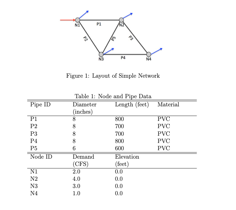
Fig. 13 Pipe network for

1. Make a table that lists each node name, node elevation, and the resultant pressure in U.S. Customary units.

2. Make a table that lists each pipe name, length, diameter, roughness height, and the resultant flow rate in U.S. Customary units.

3. Determine the flow rate in each pipe of the network, for the case where the total head at Node 1 is 100 feet.

4. Determine the Darcy-Weisbach friction factor in each pipe of the network.

5. Using the results of your flow distribution, determine the head loss from Node 1 to Node 4.

6. Determine the head at Node 4

7. Identify the node with the lowest pressure in your solution.

Exercise 2 (Advanced; optional)

Modify the algorithm and script to replace Pipe 1 in the lesson example Fig. 11 with a pump with the following pump curve.

\(\begin{equation} h_p = H_{\text{shutoff}} - K_{pump}Q^2 \end{equation} \)

Starting with values of shutoff head (116’) and a pump constant (0.05) and exponent (2) to supply water to the nodes; assume the supply node is as shown and all the nodes are at elevation 100’ (thus the pump must lift 100’).

References

previous

9: Matrix Manipulation(s) using NumPy

next

11: Databases