
ENGR 1330 Computational Thinking with Data Science
Copyright © 2021 Theodore G. Cleveland and Farhang Forghanparast
Last GitHub Commit Date:
11: Databases
Fundamental Concepts
Dataframes
Read/Write to from files
Objectives
To understand the dataframe abstraction as implemented in the Pandas library(module).
To be able to access and manipulate data within a dataframe
To be able to obtain basic statistical measures of data within a dataframe
Read/Write from/to files
MS Excel-type files (.xls,.xlsx,.csv) (LibreOffice files use the MS .xml standard)
Ordinary ASCII (.txt) files
Computational Thinking Concepts
The CT concepts expressed within Databases include:
Decomposition: Break a problem down into smaller pieces; Collections of data are decomposed into their smallest usable partAbstraction: A database is an abstraction of a collection of data
Suppose we need to store a car as a collection of its parts (implying dissassembly each time we park it), such decompotion would produce a situation like the image.

If the location of each part is recorded, then we can determine if something is missing as in

In the image, the two missing parts are pretty large, and would be evident on a fully assembled car (missing front corner panel, and right rear tire. Smaller parts would be harder to track on the fully assembled object. However if we had two fully assembled cars, and when we moved them heard the tink-tink-tink of a ball bearing bouncing on the floor, we would know something is missing - a query of the database to find where all the balls are supposed to be will help us figure out which car is incomplete.
In other contexts you wouldn’t want to have to take your car apart and store every piece separately whenever you park it in the garage. In that case, you would want to store your car as a single entry in the database (garage), and access its pieces through it (used car parts are usually sourced from fully assembled cars.
The U.S. Airforce keeps a lot of otherwise broken aircraft for parts replacement. As a part is removed it is entered into a database “a transaction” so they know that part is no longer in the broken aircraft lot but in service somewhere. So the database may locate a part in a bin in a hangar or a part that is residing in an assembled aircraft. In either case, the hangar (and parts bin) as well as the broken aircarft are both within the database schema - an abstraction.

And occassionally they grab a whole airframe

Databases
Databases are containers for data. A public library stores books, hence we could legitimately state that a library is a database of books. But strictly defined, databases are computer structures that save, organize, protect, and deliver data. A system that contains and manipulates databases is called a database management system, or DBMS.
A database can be thought of as a kind of electronic filing cabinet; it contains digitized information (“data”), which is kept in persistent storage of some kind. Users can insert new information into the database, and delete, change, or retrieve existing information in the database, by issuing requests or commands to the software that manages the database—which is to say, the database management system (DBMS).
In practice those user requests to the DBMS can be formulated in a variety of different ways (e.g., by pointing and clicking with a mouse). For our purposes, however, it’s more convenient to assume they’re expressed in the form of simple text strings in some formal language. Given a human resources database, for example, we might write:
EMP WHERE JOB = 'Programmer'
And this expression represents a retrieval request—more usually known as a query for employee information for employees whose job title is ‘Programmer’. A query submission and responce is called a transaction.
Database Types
The simplest form of databases is a text database. When data are organized in a text file in rows and columns, it can be used to store, organize, protect, and retrieve data. Saving a list of names in a file, starting with first name and followed by last name, would be a simple database. Each row of the file represents a record. You can update records by changing specific names, you can remove rows by deleting lines, and you can add new rows by adding new lines. The term “flat-file” database is a typical analog.
Desktop database programs are another type of database that’s more complex than a flat-file text database yet still intended for a single user. A Microsoft Excel spreadsheet or Microsoft Access database are good examples of desktop database programs. These programs allow users to enter data, store it, protect it, and retrieve it when needed. The benefit of desktop database programs over text databases is the speed of changing data, and the ability to store comparatively large amounts of data while keeping performance of the system manageable.
Relational databases are the most common database systems. A relational database contains multiple tables of data with rows and columns that relate to each other through special key fields. These databases are more flexible than flat file structures, and provide functionality for reading, creating, updating, and deleting data. Relational databases use variations of Structured Query Language (SQL) - a standard user application that provides an easy programming interface for database interaction.
Some examples of Relational Database Management Systems (RDMS) are SQL Server, Oracle Database, Sybase, Informix, and MySQL. The relational database management systems (RDMS) exhibit superior performance for managing large collections of for multiple users (even thousands!) to work with the data at the same time, with elaborate security to protect the data. RDBMS systems still store data in columns and rows, which in turn make up tables. A table in RDBMS is like a spreadsheet, or any other flat-file structure. A set of tables makes up a schema. A number of schemas create a database.
Emergent structures for storing data today are NoSQL and object-oriented databases. These do not follow the table/row/column approach of RDBMS. Instead, they build bookshelves of elements and allow access per bookshelf. So, instead of tracking individual words in books, NoSQL and object-oriented databases narrow down the data you are looking for by pointing you to the bookshelf, then a mechanical assistant works with the books to identify the exact word you are looking for.
Relational Database Concepts
The figure below shows sample values for a typical database, having to do with suppliers, parts, and shipments (of parts by suppliers).
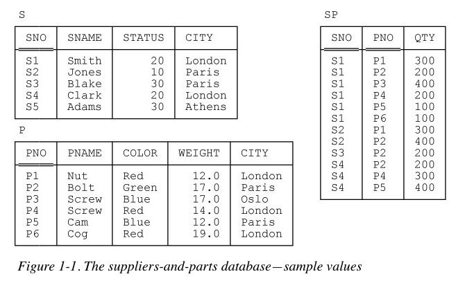
Observe that this database contains three files, or tables. The tables are named S, P, and SP, respectively, and since they’re tables they’re made up of rows and columns (in conventional file terms, the rows correspond to records of the file in question and the columns to fields). They’re meant to be understood as follows:
Table S represents suppliers under contract. Each supplier has one supplier number (SNO), unique to that supplier; one name (SNAME), not necessarily unique (though the sample values shown in Figure 1-1 do happen to be unique); one status value (STATUS); and one location (CITY). Note: In the rest of this book I’ll abbreviate “suppliers under contract,” most of the time, to just suppliers.
Table P represents kinds of parts. Each kind of part has one part number (PNO), which is unique; one name (PNAME); one color (COLOR); one weight (WEIGHT); and one location where parts of that kind are stored (CITY). Note: In the rest of this book I’ll abbreviate “kinds of parts,” most of the time, to just parts.
Table SP represents shipments—it shows which parts are shipped, or supplied, by which suppliers. Each shipment has one supplier number (SNO); one part number (PNO); and one quantity (QTY). Also, there’s at most one shipment at any given time for a given supplier and given part, and so the combination of supplier number and part number is unique to any given shipment.
Real databases tend to be much more complicated than this “toy” example. However we can make useful observations; these three tables are our schema (our framework for lack of a better word), and at this point is also our only schema, hence it is the PartsIsParts database (we have just named the database here)
Dataframe-type Structure using primative python
First lets construct a dataframe like objects using python primatives, and the PartsIsParts database schema
parts = [['PNO','PNAME','COLOR','WEIGHT','CITY'],
         ['P1','Nut','Red',12.0,'London'],
         ['P2','Bolt','Green',17.0,'Paris'],
         ['P3','Screw','Blue',17.0,'Oslo'],
         ['P4','Screw','Red',14.0,'London'],
         ['P5','Cam','Blue',12.0,'Paris'],
         ['P6','Cog','Red',19.0,'London'],]
suppliers = [['SNO','SNAME','STATUS','CITY'],
             ['S1','Smith',20,'London'],
             ['S2','Jones',10,'Paris'],
             ['S3','Blake',30,'Paris'],
             ['S4','Clark',20,'London'],
             ['S5','Adams',30,'Athens']]
shipments = [['SNO','PNO','QTY'],
             ['S1','P1',300],
             ['S1','P2',200],
             ['S1','P3',400],
             ['S1','P4',200],
             ['S1','P5',100],
             ['S1','P6',100],
             ['S2','P1',300],
             ['S2','P2',400],
             ['S3','P2',200],
             ['S4','P2',200],
             ['S4','P4',300],
             ['S4','P5',400]]
Lets examine some things:
In each table there are columns, these are called fields. There are also rows, these are called records. Hidden from view is a unique record identifier for each record, each table.
Now lets query our database, lets list all parts whose weight is less than 13 - how do we proceede?
We have to select the right table
We have to construct a search to find all instances of parts with weight less than 13
Print the result
For the toy problem not too hard
for i in range(1,len(parts)):
    if parts[i][3] < 13.0 :
        print(parts[i])
['P1', 'Nut', 'Red', 12.0, 'London']
['P5', 'Cam', 'Blue', 12.0, 'Paris']
Now lets query our database, lets list all parts whose weight is less than 13 - but only list the part number, color, and city
We have to select the right table
We have to construct a search to find all instances of parts with weight less than 13
Print the list slice with the requesite information
For the toy problem still not too hard, but immediately we see if this keeps up its going to get kind of tricky fast!; Also it would be nice to be able to refer to a column by its name.
for i in range(1,len(parts)):
    if parts[i][3] < 13.0 :
        print(parts[i][0],parts[i][2],parts[i][4]) # slice the sublist
P1 Red London
P5 Blue Paris
Now lets modify contents of a table. Lets delete all instances of suppliers with status 10. Then for remaining suppliers elevate their status by 5.
Again
We have to select the right table
We have to construct a search to find all instances of status equal to 10
If not equal to 10, copy the row, otherwise skip
Delete original table, and rename the temporary table
temp=[]
for i in range(len(suppliers)):
    print(suppliers[i])
for i in range(0,len(suppliers)):
    if suppliers[i][2] == 10 :
        continue
    else:
        temp.append(suppliers[i]) # slice the sublist
suppliers = temp # attempt to rewrite the original
for i in range(len(suppliers)):
    print(suppliers[i])
['SNO', 'SNAME', 'STATUS', 'CITY']
['S1', 'Smith', 20, 'London']
['S2', 'Jones', 10, 'Paris']
['S3', 'Blake', 30, 'Paris']
['S4', 'Clark', 20, 'London']
['S5', 'Adams', 30, 'Athens']
['SNO', 'SNAME', 'STATUS', 'CITY']
['S1', 'Smith', 20, 'London']
['S3', 'Blake', 30, 'Paris']
['S4', 'Clark', 20, 'London']
['S5', 'Adams', 30, 'Athens']
Now suppose we want to find how many parts are coming from London, our query gets more complex, but still manageable.
temp=[]
for i in range(0,len(suppliers)):
    if suppliers[i][3] == 'London' :
        temp.append(suppliers[i][0]) # get supplier code from london
    else:
        continue

howmany = 0 # keep count
for i in range(0,len(shipments)):
    for j in range(len(temp)):
        if shipments[i][0] == temp[j]:
            howmany = howmany + shipments[i][2]
        else:
            continue

print(howmany)
2200
Instead of writing all our own scripts, unique to each database the python community created a module called Pandas, so named because most things in the world are made in China, and their national critter is a Panda Bear (actually the name is a contraction of PANel DAta Structure’ or something close to that.
So to build these queries in an easier fashion - lets examine pandas.
The pandas module
About Pandas
How to install
Anaconda
JupyterHub/Lab (on Linux)
JupyterHub/Lab (on MacOS)
JupyterHub/Lab (on Windoze)
The Dataframe
Primatives
Using Pandas
Create, Modify, Delete datagrames
Slice Dataframes
Conditional Selection
Synthetic Programming (Symbolic Function Application)
Files
Access Files from a remote Web Server
Get file contents
Get the actual file
Adaptations for encrypted servers (future semester)
About Pandas:
Pandas is the core library for dataframe manipulation in Python. It provides a high-performance multidimensional array object, and tools for working with these arrays. The library’s name is derived from the term ‘Panel Data’. If you are curious about Pandas, this cheat sheet is recommended: https://pandas.pydata.org/Pandas_Cheat_Sheet.pdf
Data Structure
The Primary data structure is called a dataframe. It is an abstraction where data are represented as a 2-dimensional mutable and heterogenous tabular data structure; much like a Worksheet in MS Excel. The structure itself is popular among statisticians and data scientists and business executives.
According to the marketing department “Pandas Provides rich data structures and functions designed to make working with data fast, easy, and expressive. It is useful in data manipulation, cleaning, and analysis; Pandas excels in performance and productivity “
The Dataframe
A data table is called a DataFrame in pandas (and other programming environments too). The figure below from https://pandas.pydata.org/docs/getting_started/index.html illustrates a dataframe model:
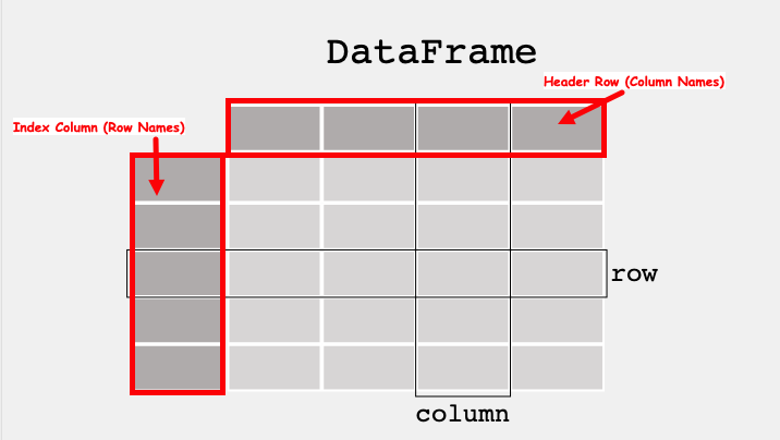
Each column and each row in a dataframe is called a series, the header row, and index column are special.
Like MS Excel we can query the dataframe to find the contents of a particular cell using its row name and column name, or operate on entire rows and columns
To use pandas, we need to import the module.
Computational Thinking Concepts
The CT concepts expressed within Pandas include:
Decomposition: Data interpretation, manipulation, and analysis of Pandas dataframes is an act of decomposition – although the dataframes can be quite complex.Abstraction: The dataframe is a data representation abstraction that allows for placeholder operations, later substituted with specific contents for a problem; enhances reuse and readability. We leverage the principle of algebraic replacement using these abstractions.Algorithms: Data interpretation, manipulation, and analysis of dataframes are generally implemented as part of a supervisory algorithm.
Module Set-Up
In principle, Pandas should be available in a default Anaconda install
You should not have to do any extra installation steps to install the library in Python
You do have to import the library in your scripts
How to check
Simply open a code cell and run
import pandasif the notebook does not protest (i.e. pink block of error), the youis good to go.
import pandas
If you do get an error, that means that you will have to install using conda or pip; you are on-your-own here! On the content server the process is:
Open a new terminal from the launcher
Change to root user
suthen enter the root passwordsudo -H /opt/jupyterhib/bin/python3 -m pip install pandasWait until the install is complete; for security, user
compthinkis not in thesudogroupVerify the install by trying to execute
import pandasas above.
The process above will be similar on a Macintosh, or Windows if you did not use an Anaconda distribution. Best is to have a sucessful anaconda install, or go to the GoodJobUntilMyOrgansGetHarvested.
If you have to do this kind of install, you will have to do some reading, some references I find useful are:
https://jupyterlab.readthedocs.io/en/stable/user/extensions.html
https://jupyterhub.readthedocs.io/en/stable/installation-guide-hard.html (This is the approach on the content server which has a functioning JupyterHub)
#%reset -f
Now lets repeat the example using Pandas, here we will reuse the original lists, so there is some extra work to get the structures just so
import pandas
partsdf = pandas.DataFrame(parts)
partsdf.set_axis(parts[0][:],axis=1,inplace=True)  # label the columns
partsdf.drop(0, axis=0, inplace = True) # remove the first row that held the column names
partsdf
| PNO | PNAME | COLOR | WEIGHT | CITY | |
|---|---|---|---|---|---|
| 1 | P1 | Nut | Red | 12 | London |
| 2 | P2 | Bolt | Green | 17 | Paris |
| 3 | P3 | Screw | Blue | 17 | Oslo |
| 4 | P4 | Screw | Red | 14 | London |
| 5 | P5 | Cam | Blue | 12 | Paris |
| 6 | P6 | Cog | Red | 19 | London |
suppliersdf = pandas.DataFrame(suppliers)
suppliersdf.set_axis(suppliers[0][:],axis=1,inplace=True)  # label the columns
suppliersdf.drop(0, axis=0, inplace = True) # remove the first row that held the column names
suppliersdf
| SNO | SNAME | STATUS | CITY | |
|---|---|---|---|---|
| 1 | S1 | Smith | 20 | London |
| 2 | S3 | Blake | 30 | Paris |
| 3 | S4 | Clark | 20 | London |
| 4 | S5 | Adams | 30 | Athens |
shipmentsdf = pandas.DataFrame(shipments)
shipmentsdf.set_axis(shipments[0][:],axis=1,inplace=True)  # label the columns
shipmentsdf.drop(0, axis=0, inplace = True) # remove the first row that held the column names
shipmentsdf
| SNO | PNO | QTY | |
|---|---|---|---|
| 1 | S1 | P1 | 300 |
| 2 | S1 | P2 | 200 |
| 3 | S1 | P3 | 400 |
| 4 | S1 | P4 | 200 |
| 5 | S1 | P5 | 100 |
| 6 | S1 | P6 | 100 |
| 7 | S2 | P1 | 300 |
| 8 | S2 | P2 | 400 |
| 9 | S3 | P2 | 200 |
| 10 | S4 | P2 | 200 |
| 11 | S4 | P4 | 300 |
| 12 | S4 | P5 | 400 |
Now lets learn about our three dataframes
partsdf.shape # this is a method to return shape, notice no argument list i.e. no ()
(6, 5)
suppliersdf.shape
(4, 4)
shipmentsdf.shape
(12, 3)
partsdf['COLOR'] #Selecing a single column
1      Red
2    Green
3     Blue
4      Red
5     Blue
6      Red
Name: COLOR, dtype: object
partsdf[['COLOR','CITY']] #Selecing a multiple columns - note the names are supplied as a list
| COLOR | CITY | |
|---|---|---|
| 1 | Red | London |
| 2 | Green | Paris |
| 3 | Blue | Oslo |
| 4 | Red | London |
| 5 | Blue | Paris |
| 6 | Red | London |
partsdf.loc[[5,6]] #Selecing rows based on label via loc[ ] indexer using row indices - note supplied as a list
| PNO | PNAME | COLOR | WEIGHT | CITY | |
|---|---|---|---|---|---|
| 5 | P5 | Cam | Blue | 12 | Paris |
| 6 | P6 | Cog | Red | 19 | London |
Now lets query our dataframes, lets list all parts whose weight is less than 13,
Recall from before:
We have to select the right table
We have to construct a search to find all instances of parts with weight less than 13
Print the list slice with the requesite information
We have to do these same activities, but the syntax is far more readable:
partsdf[partsdf['WEIGHT'] < 13] # from dataframe named partsdf, find all rows in column "WEIGHT less than 13, and return these rows"
| PNO | PNAME | COLOR | WEIGHT | CITY | |
|---|---|---|---|---|---|
| 1 | P1 | Nut | Red | 12 | London |
| 5 | P5 | Cam | Blue | 12 | Paris |
Now lets query our dataframe, lets list all parts whose weight is less than 13 - but only list the part number, color, and city
We have to select the right table
We have to construct a search to find all instances of parts with weight less than 13
Print the list slice with the requesite information
Again a more readable syntax
partsdf[partsdf['WEIGHT'] < 13][['PNO','COLOR','CITY']] # from dataframe named partsdf, find all rows in column "WEIGHT less than 13, and return part number, color, and city from these rows"
| PNO | COLOR | CITY | |
|---|---|---|---|
| 1 | P1 | Red | London |
| 5 | P5 | Blue | Paris |
head method
Returns the first few rows, useful to infer structure
shipmentsdf.head() # if you supply an argument you control how many rows are shown i.e. shipmentsdf.head(3) returns first 3 rows
| SNO | PNO | QTY | |
|---|---|---|---|
| 1 | S1 | P1 | 300 |
| 2 | S1 | P2 | 200 |
| 3 | S1 | P3 | 400 |
| 4 | S1 | P4 | 200 |
| 5 | S1 | P5 | 100 |
tail method
Returns the last few rows, useful to infer structure
shipmentsdf.tail()
| SNO | PNO | QTY | |
|---|---|---|---|
| 8 | S2 | P2 | 400 |
| 9 | S3 | P2 | 200 |
| 10 | S4 | P2 | 200 |
| 11 | S4 | P4 | 300 |
| 12 | S4 | P5 | 400 |
info method
Returns the data model (data column count, names, data types)
#Info about the dataframe

suppliersdf.info()
<class 'pandas.core.frame.DataFrame'>
Int64Index: 4 entries, 1 to 4
Data columns (total 4 columns):
 #   Column  Non-Null Count  Dtype
---  ------  --------------  -----
 0   SNO     4 non-null      object
 1   SNAME   4 non-null      object
 2   STATUS  4 non-null      object
 3   CITY    4 non-null      object
dtypes: object(4)
memory usage: 160.0+ bytes
describe method
Returns summary statistics of each numeric column.
Also returns the minimum and maximum value in each column, and the IQR (Interquartile Range).
Again useful to understand structure of the columns.
Our toy example contains limited numeric data, so describe is not too useful - but in general its super useful for engineering databases
#Statistics of the dataframe

partsdf.describe()
| PNO | PNAME | COLOR | WEIGHT | CITY | |
|---|---|---|---|---|---|
| count | 6 | 6 | 6 | 6.0 | 6 |
| unique | 6 | 5 | 3 | 4.0 | 3 |
| top | P6 | Screw | Red | 12.0 | London |
| freq | 1 | 2 | 3 | 2.0 | 3 |
Examples with “numerical” data
%reset -f
import numpy # we just reset the worksheet, so reimport the packages
import pandas
Now we shall create a proper dataframe
We will now do the same using pandas
mydf = pandas.DataFrame(numpy.random.randint(1,100,(5,4)), ['A','B','C','D','E'], ['W','X','Y','Z'])
mydf
| W | X | Y | Z | |
|---|---|---|---|---|
| A | 63 | 57 | 67 | 53 |
| B | 94 | 38 | 81 | 60 |
| C | 52 | 90 | 81 | 37 |
| D | 4 | 67 | 66 | 88 |
| E | 65 | 87 | 72 | 12 |
Getting the shape of dataframes
The shape method, which is available after the dataframe is constructed, will return the row and column rank (count) of a dataframe.
mydf.shape
(5, 4)
Appending new columns
To append a column simply assign a value to a new column name to the dataframe
mydf['new']= 'NA'
mydf
| W | X | Y | Z | new | |
|---|---|---|---|---|---|
| A | 63 | 57 | 67 | 53 | NA |
| B | 94 | 38 | 81 | 60 | NA |
| C | 52 | 90 | 81 | 37 | NA |
| D | 4 | 67 | 66 | 88 | NA |
| E | 65 | 87 | 72 | 12 | NA |
Appending new rows
This is sometimes a bit trickier but here is one way:
create a copy of a row, give it a new name.
concatenate it back into the dataframe.
newrow = mydf.loc[['E']].rename(index={"E": "X"}) # create a single row, rename the index
newtable = pandas.concat([mydf,newrow]) # concatenate the row to bottom of df - note the syntax
newtable
| W | X | Y | Z | new | |
|---|---|---|---|---|---|
| A | 63 | 57 | 67 | 53 | NA |
| B | 94 | 38 | 81 | 60 | NA |
| C | 52 | 90 | 81 | 37 | NA |
| D | 4 | 67 | 66 | 88 | NA |
| E | 65 | 87 | 72 | 12 | NA |
| X | 65 | 87 | 72 | 12 | NA |
Removing Rows and Columns
To remove a column is straightforward, we use the drop method
newtable.drop('new', axis=1, inplace = True)
newtable
| W | X | Y | Z | |
|---|---|---|---|---|
| A | 63 | 57 | 67 | 53 |
| B | 94 | 38 | 81 | 60 |
| C | 52 | 90 | 81 | 37 |
| D | 4 | 67 | 66 | 88 |
| E | 65 | 87 | 72 | 12 |
| X | 65 | 87 | 72 | 12 |
To remove a row, you really got to want to, easiest is probablty to create a new dataframe with the row removed
newtable = newtable.loc[['A','B','D','E','X']] # select all rows except C
newtable
| W | X | Y | Z | |
|---|---|---|---|---|
| A | 63 | 57 | 67 | 53 |
| B | 94 | 38 | 81 | 60 |
| D | 4 | 67 | 66 | 88 |
| E | 65 | 87 | 72 | 12 |
| X | 65 | 87 | 72 | 12 |
# or just use drop with axis specify
newtable.drop('X', axis=0, inplace = True)
newtable
| W | X | Y | Z | |
|---|---|---|---|---|
| A | 63 | 57 | 67 | 53 |
| B | 94 | 38 | 81 | 60 |
| D | 4 | 67 | 66 | 88 |
| E | 65 | 87 | 72 | 12 |
Indexing
We have already been indexing, but a few examples follow:
newtable['X'] #Selecing a single column
A    57
B    38
D    67
E    87
Name: X, dtype: int64
newtable[['X','W']] #Selecing a multiple columns
| X | W | |
|---|---|---|
| A | 57 | 63 |
| B | 38 | 94 |
| D | 67 | 4 |
| E | 87 | 65 |
newtable.loc['E'] #Selecing rows based on label via loc[ ] indexer
W    65
X    87
Y    72
Z    12
Name: E, dtype: int64
newtable
| W | X | Y | Z | |
|---|---|---|---|---|
| A | 63 | 57 | 67 | 53 |
| B | 94 | 38 | 81 | 60 |
| D | 4 | 67 | 66 | 88 |
| E | 65 | 87 | 72 | 12 |
newtable.loc[['E','D','B']] #Selecing multiple rows based on label via loc[ ] indexer
| W | X | Y | Z | |
|---|---|---|---|---|
| E | 65 | 87 | 72 | 12 |
| D | 4 | 67 | 66 | 88 |
| B | 94 | 38 | 81 | 60 |
newtable.loc[['B','E','D'],['X','Y']] #Selecting elements via both rows and columns via loc[ ] indexer
| X | Y | |
|---|---|---|
| B | 38 | 81 |
| E | 87 | 72 |
| D | 67 | 66 |
Conditional Selection
mydf = pandas.DataFrame({'col1':[1,2,3,4,5,6,7,8],
                   'col2':[444,555,666,444,666,111,222,222],
                   'col3':['orange','apple','grape','mango','jackfruit','watermelon','banana','peach']})
mydf
| col1 | col2 | col3 | |
|---|---|---|---|
| 0 | 1 | 444 | orange |
| 1 | 2 | 555 | apple |
| 2 | 3 | 666 | grape |
| 3 | 4 | 444 | mango |
| 4 | 5 | 666 | jackfruit |
| 5 | 6 | 111 | watermelon |
| 6 | 7 | 222 | banana |
| 7 | 8 | 222 | peach |
#What fruit corresponds to the number 555 in ‘col2’?

mydf[mydf['col2']==555]['col3']
1    apple
Name: col3, dtype: object
#What fruit corresponds to the minimum number in ‘col2’?

mydf[mydf['col2']==mydf['col2'].min()]['col3']
5    watermelon
Name: col3, dtype: object
Descriptor Functions
#Creating a dataframe from a dictionary

mydf = pandas.DataFrame({'col1':[1,2,3,4,5,6,7,8],
                   'col2':[444,555,666,444,666,111,222,222],
                   'col3':['orange','apple','grape','mango','jackfruit','watermelon','banana','peach']})
mydf
| col1 | col2 | col3 | |
|---|---|---|---|
| 0 | 1 | 444 | orange |
| 1 | 2 | 555 | apple |
| 2 | 3 | 666 | grape |
| 3 | 4 | 444 | mango |
| 4 | 5 | 666 | jackfruit |
| 5 | 6 | 111 | watermelon |
| 6 | 7 | 222 | banana |
| 7 | 8 | 222 | peach |
#Returns only the first five rows

mydf.head()
| col1 | col2 | col3 | |
|---|---|---|---|
| 0 | 1 | 444 | orange |
| 1 | 2 | 555 | apple |
| 2 | 3 | 666 | grape |
| 3 | 4 | 444 | mango |
| 4 | 5 | 666 | jackfruit |
info method
Returns the data model (data column count, names, data types)
#Info about the dataframe

mydf.info()
<class 'pandas.core.frame.DataFrame'>
RangeIndex: 8 entries, 0 to 7
Data columns (total 3 columns):
 #   Column  Non-Null Count  Dtype
---  ------  --------------  -----
 0   col1    8 non-null      int64
 1   col2    8 non-null      int64
 2   col3    8 non-null      object
dtypes: int64(2), object(1)
memory usage: 320.0+ bytes
describe method
Returns summary statistics of each numeric column.
Also returns the minimum and maximum value in each column, and the IQR (Interquartile Range).
Again useful to understand structure of the columns.
#Statistics of the dataframe

mydf.describe()
| col1 | col2 | |
|---|---|---|
| count | 8.00000 | 8.0000 |
| mean | 4.50000 | 416.2500 |
| std | 2.44949 | 211.8576 |
| min | 1.00000 | 111.0000 |
| 25% | 2.75000 | 222.0000 |
| 50% | 4.50000 | 444.0000 |
| 75% | 6.25000 | 582.7500 |
| max | 8.00000 | 666.0000 |
Counting and Sum methods
There are also methods for counts and sums by specific columns
mydf['col2'].sum() #Sum of a specified column
3330
The unique method returns a list of unique values (filters out duplicates in the list, underlying dataframe is preserved)
mydf['col2'].unique() #Returns the list of unique values along the indexed column
array([444, 555, 666, 111, 222])
The nunique method returns a count of unique values
mydf['col2'].nunique() #Returns the total number of unique values along the indexed column
5
The value_counts() method returns the count of each unique value (kind of like a histogram, but each value is the bin)
mydf['col2'].value_counts() #Returns the number of occurences of each unique value
222    2
444    2
666    2
111    1
555    1
Name: col2, dtype: int64
Using functions in dataframes - symbolic apply
The power of Pandas is an ability to apply a function to each element of a dataframe series (or a whole frame) by a technique called symbolic (or synthetic programming) application of the function.
This employs principles of pattern matching, abstraction, and algorithm development; a holy trinity of Computational Thinning.
It’s somewhat complicated but quite handy, best shown by an example:
def times2(x):  # A prototype function to scalar multiply an object x by 2
    return(x*2)

print(mydf)
print('Apply the times2 function to col2')
mydf['reallynew'] = mydf['col2'].apply(times2) #Symbolic apply the function to each element of column col2, result is another dataframe
   col1  col2        col3
0     1   444      orange
1     2   555       apple
2     3   666       grape
3     4   444       mango
4     5   666   jackfruit
5     6   111  watermelon
6     7   222      banana
7     8   222       peach
Apply the times2 function to col2
mydf
| col1 | col2 | col3 | reallynew | |
|---|---|---|---|---|
| 0 | 1 | 444 | orange | 888 |
| 1 | 2 | 555 | apple | 1110 |
| 2 | 3 | 666 | grape | 1332 |
| 3 | 4 | 444 | mango | 888 |
| 4 | 5 | 666 | jackfruit | 1332 |
| 5 | 6 | 111 | watermelon | 222 |
| 6 | 7 | 222 | banana | 444 |
| 7 | 8 | 222 | peach | 444 |
Sorts
mydf.sort_values('col2', ascending = True) #Sorting based on columns
| col1 | col2 | col3 | reallynew | |
|---|---|---|---|---|
| 5 | 6 | 111 | watermelon | 222 |
| 6 | 7 | 222 | banana | 444 |
| 7 | 8 | 222 | peach | 444 |
| 0 | 1 | 444 | orange | 888 |
| 3 | 4 | 444 | mango | 888 |
| 1 | 2 | 555 | apple | 1110 |
| 2 | 3 | 666 | grape | 1332 |
| 4 | 5 | 666 | jackfruit | 1332 |
mydf.sort_values('col3', ascending = True) #Lexiographic sort
| col1 | col2 | col3 | reallynew | |
|---|---|---|---|---|
| 1 | 2 | 555 | apple | 1110 |
| 6 | 7 | 222 | banana | 444 |
| 2 | 3 | 666 | grape | 1332 |
| 4 | 5 | 666 | jackfruit | 1332 |
| 3 | 4 | 444 | mango | 888 |
| 0 | 1 | 444 | orange | 888 |
| 7 | 8 | 222 | peach | 444 |
| 5 | 6 | 111 | watermelon | 222 |
Aggregating (Grouping Values) dataframe contents
#Creating a dataframe from a dictionary

data = {
    'key' : ['A', 'B', 'C', 'A', 'B', 'C'],
    'data1' : [1, 2, 3, 4, 5, 6],
    'data2' : [10, 11, 12, 13, 14, 15],
    'data3' : [20, 21, 22, 13, 24, 25]
}

mydf1 = pandas.DataFrame(data)
mydf1
| key | data1 | data2 | data3 | |
|---|---|---|---|---|
| 0 | A | 1 | 10 | 20 |
| 1 | B | 2 | 11 | 21 |
| 2 | C | 3 | 12 | 22 |
| 3 | A | 4 | 13 | 13 |
| 4 | B | 5 | 14 | 24 |
| 5 | C | 6 | 15 | 25 |
# Grouping and summing values in all the columns based on the column 'key'

mydf1.groupby('key').sum()
| data1 | data2 | data3 | |
|---|---|---|---|
| key | |||
| A | 5 | 23 | 33 |
| B | 7 | 25 | 45 |
| C | 9 | 27 | 47 |
# Grouping and summing values in the selected columns based on the column 'key'

mydf1.groupby('key')[['data1', 'data2']].sum()
| data1 | data2 | |
|---|---|---|
| key | ||
| A | 5 | 23 |
| B | 7 | 25 |
| C | 9 | 27 |
Filtering out missing values
Filtering and cleaning are often used to describe the process where data that does not support a narrative is removed ;typically for maintenance of profit applications, if the data are actually missing that is common situation where cleaning is justified.
#Creating a dataframe from a dictionary

df = pandas.DataFrame({'col1':[1,2,3,4,None,6,7,None],
                   'col2':[444,555,None,444,666,111,None,222],
                   'col3':['orange','apple','grape','mango','jackfruit','watermelon','banana','peach']})
df
| col1 | col2 | col3 | |
|---|---|---|---|
| 0 | 1.0 | 444.0 | orange |
| 1 | 2.0 | 555.0 | apple |
| 2 | 3.0 | NaN | grape |
| 3 | 4.0 | 444.0 | mango |
| 4 | NaN | 666.0 | jackfruit |
| 5 | 6.0 | 111.0 | watermelon |
| 6 | 7.0 | NaN | banana |
| 7 | NaN | 222.0 | peach |
Below we drop any row that contains a NaN code.
df_dropped = df.dropna()
df_dropped
| col1 | col2 | col3 | |
|---|---|---|---|
| 0 | 1.0 | 444.0 | orange |
| 1 | 2.0 | 555.0 | apple |
| 3 | 4.0 | 444.0 | mango |
| 5 | 6.0 | 111.0 | watermelon |
Below we replace NaN codes with some value, in this case 0
df_filled1 = df.fillna(0)
df_filled1
| col1 | col2 | col3 | |
|---|---|---|---|
| 0 | 1.0 | 444.0 | orange |
| 1 | 2.0 | 555.0 | apple |
| 2 | 3.0 | 0.0 | grape |
| 3 | 4.0 | 444.0 | mango |
| 4 | 0.0 | 666.0 | jackfruit |
| 5 | 6.0 | 111.0 | watermelon |
| 6 | 7.0 | 0.0 | banana |
| 7 | 0.0 | 222.0 | peach |
Below we replace NaN codes with some value, in this case the mean value of of the column in which the missing value code resides.
df_filled2 = df.fillna(df.mean())
df_filled2
| col1 | col2 | col3 | |
|---|---|---|---|
| 0 | 1.000000 | 444.0 | orange |
| 1 | 2.000000 | 555.0 | apple |
| 2 | 3.000000 | 407.0 | grape |
| 3 | 4.000000 | 444.0 | mango |
| 4 | 3.833333 | 666.0 | jackfruit |
| 5 | 6.000000 | 111.0 | watermelon |
| 6 | 7.000000 | 407.0 | banana |
| 7 | 3.833333 | 222.0 | peach |
Reading a File into a Dataframe
Pandas has methods to read common file types, such as csv,xls, and json.
Ordinary text files are also quite manageable.
Specifying
engine='openpyxl'in the read/write statement is required for the xml versions of Excel (xlsx). Default is .xls regardless of file name. If you still encounter read errors, try opening the file in Excel and saving as .xls (Excel 97-2004 Workbook) or as a CSV if the structure is appropriate.
You may have to install the packages using something likesudo -H /opt/jupyterhub/bin/python3 -m pip install xlwt openpyxl xlsxwriter xlrdfrom the Anaconda Prompt interface (adjust the path to your system) or something likesudo -H /opt/conda/envs/python/bin/python -m pip install xlwt openpyxl xlsxwriter xlrd
The files in the following examples are CSV_ReadingFile.csv, Excel_ReadingFile.xlsx,
readfilecsv = pandas.read_csv('CSV_ReadingFile.csv')  #Reading a .csv file
print(readfilecsv)
    a   b   c   d
0   0   1   2   3
1   4   5   6   7
2   8   9  10  11
3  12  13  14  15
Similar to reading and writing .csv files, you can also read and write .xslx files as below (useful to know this)
readfileexcel = pandas.read_excel('Excel_ReadingFile.xlsx', sheet_name='Sheet1', engine='openpyxl') #Reading a .xlsx file
print(readfileexcel)
   Unnamed: 0   a   b   c   d
0           0   0   1   2   3
1           1   4   5   6   7
2           2   8   9  10  11
3           3  12  13  14  15
Writing a dataframe to file
#Creating and writing to a .csv file
readfilecsv = pandas.read_csv('CSV_ReadingFile.csv')
readfilecsv.to_csv('CSV_WritingFile1.csv') # write to local directory
readfilecsv = pandas.read_csv('CSV_WritingFile1.csv') # read the file back
print(readfilecsv)
   Unnamed: 0   a   b   c   d
0           0   0   1   2   3
1           1   4   5   6   7
2           2   8   9  10  11
3           3  12  13  14  15
#Creating and writing to a .csv file by excluding row labels
readfilecsv = pandas.read_csv('CSV_ReadingFile.csv')
readfilecsv.to_csv('CSV_WritingFile2.csv', index = False)
readfilecsv = pandas.read_csv('CSV_WritingFile2.csv')
print(readfilecsv)
    a   b   c   d
0   0   1   2   3
1   4   5   6   7
2   8   9  10  11
3  12  13  14  15
#Creating and writing to a .xls file
readfileexcel = pandas.read_excel('Excel_ReadingFile.xlsx', sheet_name='Sheet1', engine='openpyxl')
readfileexcel.to_excel('Excel_WritingFile.xlsx', sheet_name='Sheet1' , index = False, engine='openpyxl')
readfileexcel = pandas.read_excel('Excel_WritingFile.xlsx', sheet_name='Sheet1', engine='openpyxl')
print(readfileexcel)
   Unnamed: 0   a   b   c   d
0           0   0   1   2   3
1           1   4   5   6   7
2           2   8   9  10  11
3           3  12  13  14  15
References
Overland, B. (2018). Python Without Fear. Addison-Wesley ISBN 978-0-13-468747-6.
Grus, Joel (2015). Data Science from Scratch: First Principles with Python O’Reilly Media. Kindle Edition.
Precord, C. (2010) wxPython 2.8 Application Development Cookbook Packt Publishing Ltd. Birmingham , B27 6PA, UK ISBN 978-1-849511-78-0.
Johnson, J. (2020). Python Numpy Tutorial (with Jupyter and Colab). Retrieved September 15, 2020, from https://cs231n.github.io/python-numpy-tutorial/
Willems, K. (2019). (Tutorial) Python NUMPY Array TUTORIAL. Retrieved September 15, 2020, from https://www.datacamp.com/community/tutorials/python-numpy-tutorial?utm_source=adwords_ppc
Willems, K. (2017). NumPy Cheat Sheet: Data Analysis in Python. Retrieved September 15, 2020, from https://www.datacamp.com/community/blog/python-numpy-cheat-sheet
W3resource. (2020). NumPy: Compare two given arrays. Retrieved September 15, 2020, from https://www.w3resource.com/python-exercises/numpy/python-numpy-exercise-28.php
Sorting https://www.programiz.com/python-programming/methods/list/sort
https://www.oreilly.com/library/view/relational-theory-for/9781449365431/ch01.html
https://realpython.com/pandas-read-write-files/#using-pandas-to-write-and-read-excel-files
Laboratory 11
Examine (click) Laboratory 11 as a webpage at Laboratory 11.html
Download (right-click, save target as …) Laboratory 11 as a jupyterlab notebook from Laboratory 11.ipynb
Exercise Set 11
Examine (click) Exercise Set 11 as a webpage at Exercise 11.html
Download (right-click, save target as …) Exercise Set 11 as a jupyterlab notebook at Exercise Set 11.ipynb