Download this page as a jupyter notebook at Lab 9-TH

Laboratory 9: Matrices a Blue Pill Approach

LAST NAME, FIRST NAME

R00000000

ENGR 1330 Laboratory 9 - Homework

# Preamble script block to identify host, user, and kernel
import sys
! hostname
! whoami
print(sys.executable)
print(sys.version)
print(sys.version_info)

atomickitty
sensei
/opt/jupyterhub/bin/python3
3.8.10 (default, Jun  2 2021, 10:49:15) 
[GCC 9.4.0]
sys.version_info(major=3, minor=8, micro=10, releaselevel='final', serial=0)

Numpy Cheat Sheet(s)

Numpy is the core library for scientific computing in Python. It provides a high-performance multidimensional array object, and tools for working with these arrays. The library’s name is short for “Numeric Python” or “Numerical Python”.

A pdf file of a summary sheet (you need to download): https://s3.amazonaws.com/assets.datacamp.com/blog_assets/Numpy_Python_Cheat_Sheet.pdf

or the graphic below (same information):

---

Exercise 1: Going down to Southpark .... ?

Using the names below:

"Cartman, Kenny, Kyle, Stan, Butters, Wendy, Chef, Mr. Mackey, Randy, Sharon, Sheila, Towelie"

A) Create a 3x4 array and print it out
B) Sort the array alphabetically by column and print it out
C) From the sorted array, slice out a 2x2 array with ('Cartman, Randy, Sharon, Wendy'), and print it out

#import numpy
# make an arry of names
# print array
# sort and print sorted array
# slice and print sliced array

---

Exercise 2: A Numpy Playground

• Step1: Create a 2x5 array with [0,1,2,3,4,5,6,7,8,9] and name it "Array1"
• Step2: Extract all the odd numbers of "Array1" and store them in a new array: "Array2"
• Step3: In "Array1" replace 0,5, and 9 with 100,500, and 900.
• Step4: Add three other odd numbers to "Array2"
• Step5: Calculate the average of "Array2"
• Step6: Take "Array2" to the power of 5 and print the result.

#import numpy
# create and print array1
# create and print array2
# make replacements, print result
# Add three other odd numbers to "Array2"
# Calculate the average of "Array2"
# Take "Array2" to the power of 5 and print the result. 

---

Exercise 3:

• Step1: Create a 1D Numpy array of all the numbers in your R-number: R######## | It should have eight numbers
• Step2: Create another 1D array by multiplying the previous array by 2
• Step3: Create another 1D array by multiplying the first array by 5

# import numpy 
# Create a 1D Numpy array of all the numbers in your R-number
# Create another 1D array by multiplying the previous array by 2
# Create another 1D array by multiplying the first array by 5

---

You will also find this link helpful for the next two exercises: https://www.codecademy.com/learn/learn-linear-algebra/modules/math-ds-linear-algebra/cheatsheet

Exercise 4

Consider the linear system given by

$$\mathbf{A} \cdot \mathbf{x} = \mathbf{B}$$

where

\begin{gather} \mathbf{A}= \begin{pmatrix} 8.17\times10^6 & 0 &-0.5\times10^6\\ -1.5\times10^6 & 7.21\times10^6 & 0 \\ 0 & -1.5\times10^6 & 11.5\times10^6 \\ \end{pmatrix} ~\mathbf{b}= \begin{pmatrix} 2.0\times10^9 \\ 4.0\times10^9 \\ 1.0\times10^9 \\ \end{pmatrix} \end{gather}

Use numpy and linalg methods to find x

# import numpy 
# create A 
# create B
# x = Ainv times B
# print result

---

Exercise 5.

Consider the steady-state reactor system with feedback as shown below:

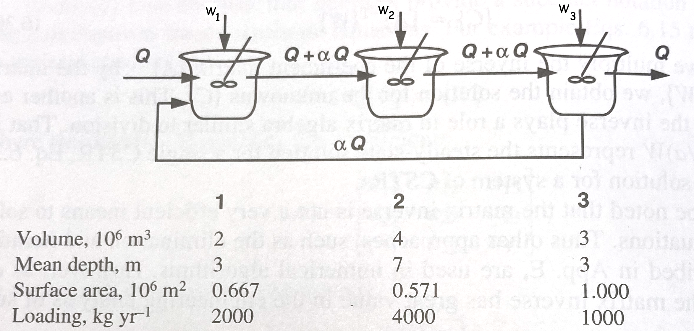
A mass balance of the system assuming complete mixing in each reactor (pond, lake, vat, ...) is

\begin{gather} \begin{matrix} W_1 = & (Q+\alpha Q + v A_1) \times C_1 & + 0 \times C_2 &- \alpha Q \times C_3\\ W_2 = & -(Q+\alpha Q) \times C_1 & + (Q+\alpha Q + v A_2) \times C_2 & 0 \times C_3 \\ W_3 = & 0 \times C_1 & - (Q+\alpha Q)\times C_2 & +(Q+\alpha Q + v A_3) \times C_3\\ \end{matrix} \end{gather}

where $W_i$ is the loading in kilograms/year , $A_i$ is the reactor surface area in $10^6$ meters squared, $v$ is the settling rate in each reactor in meters/year, $\alpha$ is the recycle fraction, and $Q$ is the volumetric flow rate through the system. The unknown values are the constituient concentrations $C_i$ in each reactor.

Decomposing the system of equations above into a Matrix-vector system $\mathbf{A} \cdot \mathbf{C} = \mathbf{W}$, where $\mathbf{A}$ is the coefficient matrix (which we will build using $Q$,$\alpha$, and $v A_i$), $\mathbf{C}$ is the vector of unknown concentrations of the constituients, and $\mathbf{W}$ is the loading vector yields:

\begin{gather} \begin{pmatrix} (Q+\alpha Q + v A_1) & + 0 &- \alpha Q \\ -(Q+\alpha Q) & + (Q+\alpha Q + v A_2) & 0 \\ 0 & - (Q+\alpha Q)& +(Q+\alpha Q + v A_3) \\ \end{pmatrix} \cdot \begin{pmatrix} C_1 \\ C_2 \\ C_3 \\ \end{pmatrix} ~=~ \begin{pmatrix} W_1 \\ W_2 \\ W_3 \\ \end{pmatrix} \end{gather}

Complete a script that constructs $\mathbf{A}$ given $Q=1\times10^6$ cubic meters/year, $\alpha$ = 0.5, and $v$ = 10 meters/year. Estimate the reactor constituient concentrations in parts per million (milligrams).

Now repeat the computation with $\alpha$ = 0.0

# import numpy
# create constants and properties arrays
# get units correct
# Load = Load*1e6 #Load in milligrams 
# Area = Area*1e6 #Area in million squre meters
# construct the coefficient array
# invert and solve for c
# print result

# import numpy
# create constants and properties arrays - change to alpha=0
# get units correct
# Load = Load*1e6 #Load in milligrams 
# Area = Area*1e6 #Area in million squre meters
# construct the coefficient array
# invert and solve for c
# print result