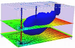
3D - Advection-Dispersion, Finite-Area, Constant Production (Injection) Source
The sketch depicts a planar source zone Y units wide and Z units tall, centered at (0,0,0).

The analytical model (Domenico and Robbins, 1985) is obtained by convolution of instantaneous sources (described in detail in Yuan, 1995):
\[ C(x,y,t) = \frac{C_0}{8} \cdot \textit{erfc}[\frac{(x - v t) }{ (2 \sqrt{D_x t))}}] \cdot [\textit{erf}(\frac{(y + \frac{Y}{2}) }{ (2 \sqrt{\frac{D_y}{v} x))}}) - \textit{erf} (\frac{(y - \frac{Y}{2}) }{ (2 \sqrt{\frac{D_y}{v} x))}})] \cdot [\textit{erf}(\frac{(z + \frac{Z}{2}) }{ (2 \sqrt{\frac{D_z}{v} x))}}) - \textit{erf} (\frac{(z - \frac{Z}{2}) }{ (2 \sqrt{\frac{D_z}{v} x))}})]\]
Note
This solution is identical to Equation 6.33, with \(\lambda = 0\), \(R = 1\).
A prototype function is
def c3dad(conc0, distx, disty, distz, lenX, lenY, lenZ, dispx, dispy, dispz, velocity, etime):
    import math
    from scipy.special import erf, erfc # scipy needs to already be loaded into the kernel
    # Constant of integration
    term1 = conc0 / 8.0

    # Centerline axis solution
    arg1 = (distx - velocity*etime) / (2*math.sqrt(dispx*velocity*etime)) #dispx is dispersivity
    term2 = erfc(arg1)

    # Off-axis solution, Y direction
#    arg2 = 2.0 * math.sqrt(dispy*distx / velocity)
    arg2 = 2.0 * math.sqrt(dispy*distx) #dispy is dispersivity
    arg3 = disty + 0.5*lenY
    arg4 = disty - 0.5*lenY
    term3 = erf(arg3 / arg2) - erf(arg4 / arg2)

    # Off-axis solution, Z direction
#    arg5 = 2.0 * math.sqrt(dispz*distx / velocity)
    arg5 = 2.0 * math.sqrt(dispz*distx) #dispz is dispersivity
    arg6 = distz + 0.5*lenZ
    arg7 = distz - 0.5*lenZ
    term4 = erf(arg6 / arg5) - erf(arg7 / arg5)

    # Convolve the solutions
    c3dad = term1 * term2 * term3 * term4
    return c3dad
Note
This is 3D part is incomplete. Needs
An example
Script to render an xyz density plot
