Sample Collection and Data Analysis
Sampling is a crucial step in assessing groundwater contamination. The objective is to obtain representative samples that accurately reflect the water quality and the presence of contaminants. Here are some key considerations in sample collection:
Sampling Locations: Careful selection of sampling locations is vital. These sites should be strategically chosen based on hydrogeological knowledge, proximity to potential contamination sources, and historical data. Monitoring wells, springs, or nearby surface water bodies can be appropriate locations.
Sampling Depth: Groundwater can exhibit vertical variability in its quality. Thus, samples should be collected at various depths to assess the full spectrum of contamination.
Sampling Frequency: Regular and consistent sampling over time is essential to track changes in groundwater quality. Seasonal variations and short-term fluctuations can impact the data.
Sample Containers: Choosing appropriate containers is critical to preserve the integrity of the samples. Containers must be clean, made of inert materials, and properly labeled.
Once samples are collected, thorough data analysis is imperative to draw meaningful conclusions about groundwater quality and contamination. Several steps are involved in this process:
Laboratory Analysis: Samples are typically analyzed in specialized laboratories using standardized methods to detect and quantify specific contaminants. Common parameters include pH, turbidity, dissolved oxygen, and the concentration of various pollutants (e.g., heavy metals, nitrates, volatile organic compounds).
Quality Control: Quality control measures, such as blank samples and duplicates, are essential to verify the accuracy and precision of laboratory results.
Data Interpretation: The collected data need to be interpreted in the context of relevant regulations and guidelines. Comparison to established water quality standards or local regulatory limits helps identify contamination levels.
Spatial Mapping: Geographic Information Systems (GIS) can be used to create spatial maps of contamination plumes, providing a visual representation of the extent and movement of pollutants.
Trend Analysis: Over time, trends in groundwater quality should be assessed. This involves statistical techniques like trend analysis and time series modeling to identify changes in contamination levels.
Risk Assessment: The final step is assessing the potential risks associated with groundwater contamination. This involves understanding the exposure pathways and potential health impacts on the community.
Demonstrating Trend(s)
Demonstration of trends will typically employ both plotting (visual cues) and some kind of trend analysis. The methods suggested in the textbook are variations of non-parametric statistical hypothesis tests. (pp. 456-462)
Mann-Kendall Trend Test is used to determine whether or not a trend exists in time series (ordered) data. It is a non-parametric test, meaning there is no underlying assumption made about the normality of the data.
The textbook presents a tabular approach for small data sets as one would expect on a remediation site - here we present a scripting approach using python packages.
Mann-Kendall Trend Test using
mk.original_test()function
In this approach, themk.original_test()function with required parameters from the pymannkendall library to conduct the Mann-Kendall Trend test on the given data in the python programming language. To install the pymannkendall library for mk.original_test() function employpiporcondalike:
root@atomickitty:/home/sensei# sudo -H /opt/jupyterhub/bin/python3 -m pip install pymannkendall
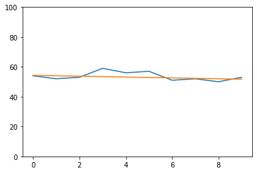
An example from https://www.geeksforgeeks.org below is used to check the install
import numpy as np
import pandas as pd
import pymannkendall as mk
import matplotlib.pyplot as plt
import statsmodels.api as sm
%matplotlib inline

gfg_data = [54, 52, 53, 59, 56, 57, 51, 52, 50, 53]

# perform Mann-Kendall Trend Test
result=mk.original_test(gfg_data,alpha=0.1)
print(result.trend)
trend_line = np.arange(len(gfg_data))*result.slope + result.intercept

#data plot
plt.plot(gfg_data)
plt.plot(trend_line)
plt.ylim(0,100)
# autocorrelation plot
#fig, ax = plt.subplots(figsize=(12, 8))
#sm.graphics.tsa.plot_acf(gfg_data, lags=7, ax=ax);
no trend
(0.0, 100.0)
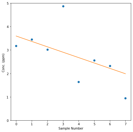
Now we have a tool, lets repeat the example on page 461 of the textbook
import numpy as np
import pandas as pd
import pymannkendall as mk
import matplotlib.pyplot as plt
import statsmodels.api as sm
%matplotlib inline
gfg_data = [3.18,3.455,3.022,4.876,1.635,2.561,2.329,0.95]

# perform Mann-Kendall Trend Test
result=mk.original_test(gfg_data,alpha=0.1)
print("Trend type: ",result.trend)
print("p-value at rejection : ",round(result.p,2))
trend_line = np.arange(len(gfg_data))*result.slope + result.intercept

#data plot
plt.figure(figsize=(7,7))
plt.plot(gfg_data,marker='o',linewidth=0)
plt.plot(trend_line)
plt.xlabel("Sample Number")
plt.ylabel("Conc. (ppm) ")
plt.ylim(0,5);
# autocorrelation plot
#fig, ax = plt.subplots(figsize=(12, 8))
#sm.graphics.tsa.plot_acf(gfg_data, lags=7, ax=ax);
Trend type:  decreasing
p-value at rejection :  0.06