Essential Groundwater Review
This essential review of groundwater should remind the reader of important aspects of:
Introduction to Groundwater including: A definition of groundwater, the importance of groundwater as a natural resource, and the distinction between surface water and groundwater.
Aquifers and Aquitards including: An explanation of aquifers and their properties, the role of aquitards in groundwater containment, types of aquifers (unconfined, confined, etc.).
Groundwater Movement: Darcy’s Law and groundwater flow, factors influencing groundwater flow rates, flow patterns in aquifers (radial flow, regional flow, etc.)
Groundwater Storage and Recharge: Methods of groundwater recharge, Groundwater storage and water table fluctuations, Sustainable groundwater management
Groundwater Flow Modeling: Overview of groundwater flow modeling, application of numerical models (MODFLOW, FEMWATER, etc.), use of models for aquifer characterization and contamination prediction
Groundwater Extraction and Wells: Types of groundwater wells (e.g., artesian wells, extraction wells), pumping tests and their significance, groundwater extraction for drinking water, remediation, and irrigation.
Porous Media (pp. 15-21)
Porous media refers to a class of materials that have interconnected void spaces or pores, allowing the flow and transport of fluids. In the context of groundwater, porous media plays a crucial role as it forms the subsurface medium through which water flows and contaminants can be transported. The properties and characteristics of the porous media significantly influence the movement of groundwater and the fate of contaminants within an aquifer.
Two fundamental properties govern behavior of fluids in a porous media:
The porosity, which represents the volume of void spaces within the material, determines the storage capacity for fluid within the porous media and affects the flow rate. Porous media with high porosity can concievably store more water, but it may also delay movement of groundwater because of reduced size of individual pores.
The permeability, which describes the ease with which fluids can flow through the porous media, depends on factors such as pore size, shape, and connectivity. High-permeability materials, like coarse sand or gravel, allow water to flow more easily, whereas low-permeability materials, like clay or silt, impede water movement. Permeability influences the speed and direction of groundwater flow, as well as the potential for contaminants to migrate through the aquifer.
Porous media also exhibits heterogeneity, meaning it can have spatial variations in these fundamental properties. This heterogeneity arises from geological processes, such as sediment deposition, compaction, and tectonic activity. Variations in porosity and permeability within a porous medium lead to complex flow patterns, preferential flow paths, and the potential for localized contaminant accumulation or dispersion. Understanding the heterogeneity of porous media is crucial for accurately predicting groundwater flow and contaminant transport.
Interactions between fluids and porous media involves various physical and chemical processes. Advection, the bulk movement of groundwater, is influenced by the permeability and hydraulic gradient. Dispersion, the spreading of solutes due to molecular diffusion and mechanical mixing, occurs as water moves through the porous medium. Adsorption refers to the attachment of contaminants to the solid surfaces of the porous media, affecting their mobility and persistence. These processes, along with others like biodegradation and chemical reactions, shape the fate and transport of contaminants in groundwater.
Saturated Zone (pp. 16-17)
The saturated zone refers to the region within the subsurface where all the available pore spaces are filled with water, creating a saturated condition. It is an important concept in groundwater hydrology and plays a crucial role in groundwater flow and contaminant transport.
The saturated zone begins at the water table, which represents the boundary between the unsaturated zone (where there is both air and water in the pore spaces) and the saturated zone (where all pore spaces are filled with water). The depth of the saturated zone can vary depending on factors such as topography, geology, and seasonality.

Within the saturated zone, groundwater flow occurs as water moves through the interconnected pore spaces under the influence of gravity. The direction and speed of groundwater flow are governed by hydraulic gradients, which are the differences in hydraulic head (a measure of the potential energy of groundwater) between different locations. The saturated zone acts as a conduit for the movement of water from areas of higher hydraulic head to areas of lower hydraulic head.
The properties of the saturated zone, such as its permeability, porosity, and heterogeneity, have a significant impact on groundwater flow. Permeability determines how easily water can move through the saturated zone. Materials with high permeability, like gravel or sand, allow for faster groundwater flow, while low-permeability materials, such as clay or shale, impede flow. Porosity, the volume of void spaces, determines the amount of water that can be stored in the saturated zone.
Heterogeneity in the saturated zone refers to variations in the properties of the porous medium, such as permeability and porosity, over space. This heterogeneity can influence the flow of groundwater by creating preferential flow paths or areas of localized flow convergence or divergence. Understanding the heterogeneity of the saturated zone is important for accurate modeling and prediction of groundwater flow patterns.
Contaminant transport also occurs within the saturated zone. Once contaminants enter the groundwater system, they can be transported through the interconnected pore spaces. The movement of contaminants is influenced by factors such as advection (bulk movement of groundwater), dispersion (spreading of contaminants due to mechanical mixing and molecular diffusion), and sorption (attachment of contaminants to solid surfaces). The saturated zone acts as a medium for the migration and dispersion of contaminants, and its properties influence the rate and extent of contaminant transport.
Unsaturated Zone (pp. 289-297)
The unsaturated zone, also known as the vadose zone or the zone of aeration, is the region within the subsurface where the pore spaces contain both air and water. In this zone, the water content is less than the total porosity of the material. The unsaturated zone extends from the land surface down to the water table, where it transitions into the saturated zone.

The unsaturated zone is characterized by a dynamic water content profile that changes over time due to factors such as precipitation, evaporation, and plant uptake. At the land surface, water infiltrates through the soil and rock layers until it reaches a point where the pore spaces are completely saturated. This point is known as the water table, which marks the transition to the saturated zone.
The movement of water in the unsaturated zone is influenced by capillary forces and gravity. Capillary forces cause water to rise in small pores against the force of gravity, allowing it to be retained in the unsaturated zone. The rate of water movement through the unsaturated zone is generally slower compared to the saturated zone due to the presence of air and the lower hydraulic conductivity of unsaturated materials.
The unsaturated zone plays a crucial role in controlling the recharge of groundwater. It acts as a buffer, allowing for the filtration, storage, and gradual release of water to the underlying aquifer. The unsaturated zone also contributes to the purification of water through processes such as filtration, adsorption, and biodegradation as water percolates through the soil and rock layers.
In terms of contaminant transport, the unsaturated zone can act as a barrier or filter, reducing the potential for contaminants to reach the groundwater system. The unsaturated materials can adsorb or retain contaminants, and the slower movement of water through this zone provides additional time for degradation or removal of contaminants.
Aquifers (pp. 18-23)
An aquifer is a geologic formation that (i) contains and (ii) transmits water in economically useful quantities under normal field conditions.
Some related terms include:
An aquitard is a geologic formation or layer that has low permeability, restricting the flow of groundwater. It acts as a barrier or confining layer that limits the movement of water between aquifers. Unlike aquifers, which are capable of storing and transmitting water, aquitards have a lower hydraulic conductivity, impeding or retarding the flow of groundwater. Aquitards can consist of various materials such as clay, silt, shale, or unconsolidated sediment, which offer limited pathways for groundwater movement. They play a crucial role in groundwater systems by confining and isolating aquifers, influencing groundwater storage, and controlling the vertical movement of water.
An aquifuge is a geologic formation or layer that is essentially impermeable to groundwater flow. Unlike aquitards, which have limited permeability, aquifuges are completely impermeable, meaning they do not allow the movement of water. Aquifuges act as barriers that prevent the flow of groundwater between aquifers and restrict the vertical or lateral movement of water. They are typically composed of dense and impermeable materials such as unfractured bedrock, solid clay, or thick layers of compacted till. Aquifuges are important in groundwater hydrology as they create boundaries or seals that confine and isolate aquifers, preventing the intermixing or contamination of groundwater between different layers.
An aquiclude is a geologic formation or layer that is completely impermeable to groundwater flow. It is similar to an aquifuge in that it acts as a barrier to the movement of water, but it differs in that it is typically much thicker and more extensive. Aquicludes are composed of highly impermeable materials, such as solid rock or dense clay, which do not allow water to pass through them. They effectively impede the flow of groundwater and can serve as long-lasting barriers between aquifers. Aquicludes are important features in groundwater systems as they help confine and isolate aquifers, preventing the vertical or lateral movement of water and maintaining the integrity of groundwater resources.
Aquifers are typically categorized as confined or unconfined; these two types of aquifers that differ in their geological characteristics and water storage conditions.

Definition:
Confined Aquifer: A confined aquifer, also known as an artesian aquifer, is an aquifer that is bounded above and below by impermeable layers, such as clay or dense rock, which confine the groundwater within a confined space.
Unconfined Aquifer: An unconfined aquifer, also called a water table aquifer, is an aquifer where the upper boundary, known as the water table, is not confined by an impermeable layer, allowing water to freely move up and down through the aquifer.
Recharge:
Confined Aquifer: Confined aquifers are typically recharged in areas where the confining layers are absent or fractured, allowing water to infiltrate from the surface. Recharge to confined aquifers can be more limited and localized.
Unconfined Aquifer: Unconfined aquifers are primarily recharged through precipitation, where water percolates through the unsaturated zone until it reaches the water table. Recharge to unconfined aquifers can occur over larger areas.
Water Storage and Pressure:
Confined Aquifer: Due to the confining layers, water in confined aquifers is under higher pressure and can be stored under artesian conditions. When a well is drilled into a confined aquifer, the water may rise above the ground level due to the pressure exerted by the confined aquifer.
Unconfined Aquifer: Water in unconfined aquifers is not under significant pressure and is stored under the water table. The height of the water table fluctuates based on factors such as recharge rates, extraction, and seasonality.
Vulnerability to Contamination:
Confined Aquifer: Confined aquifers are generally less vulnerable to contamination compared to unconfined aquifers. The presence of confining layers acts as a barrier, limiting the potential for contaminants to infiltrate the aquifer.
Unconfined Aquifer: Unconfined aquifers are more susceptible to contamination as there is no confining layer to impede the movement of contaminants. Contaminants can more easily reach the water table and potentially affect the groundwater quality.
Extraction and Well Productivity:
Confined Aquifer: Extraction of water from a confined aquifer typically yields higher well productivity due to the increased pressure within the aquifer. Wells drilled into confined aquifers can have a steady and sustained water supply.
Unconfined Aquifer: Extraction from unconfined aquifers may yield variable well productivity depending on the fluctuating water table. The yield of wells in unconfined aquifers may be influenced by seasonal variations in recharge and the proximity to other water sources.
A leaky aquifer refers to an aquifer that exhibits characteristics of both an aquifer and an aquitard. It is a geological formation that has varying degrees of permeability and acts as a partial barrier to the flow of groundwater. In a leaky aquifer, the presence of semi-permeable layers or zones with lower permeability allows some water to pass through, while also impeding or retarding the flow to some extent.
Leaky aquifers are distinct from fully confined aquifers or unconfined aquifers, as they possess intermediate characteristics. They can be seen as “leaky” due to the reduced hydraulic conductivity of the semi-permeable layers present within the aquifer system. These semi-permeable layers act as partial barriers, restricting or slowing down the movement of groundwater between different zones or layers.
The presence of leaky aquifers can have significant implications for groundwater management and hydrogeological assessments. They can influence the flow paths, distribution, and quality of groundwater within an aquifer system. Understanding the extent and properties of leaky aquifers is crucial for accurately modeling groundwater flow, assessing contaminant transport, and managing water resources effectively.
Storage
Storativity is the amount of water added to/released from storage per unit change in head per unit area of aquifer. Mechanisms of storage are draining and filling of the pore space (unconfined) and compression/decompression of the solid matrix and water (confined).
In confined aquifers the storage coefficient is denoted by the symbol \(S\). In unconfined aquifers the storage coefficient is the specific yield and is denoted by \(S_y\). The amount remaining is called the specific retention \(S_r\). The sum of these two terms is the porosity.
Transport (of Water)
The ability to convey water is measured by the permeability, in the case of water it is called the hydraulic conductivtiy. It is a combined property of porous media properties and fluid properties, the usual symbol is \(K\).
Note
The hydraulic conductivity for porous media plays the same role as the friction factor in pipe flow, which is also a combined property of pipe material and fluid properties.:::
The ability of an entire thickness of aquifer to transmit water is called the transmissivity; the usual symbol is \(T\)
Darcy’s Law
Darcy’s Law is a fundamental principle in hydrogeology that describes the movement of groundwater through porous media and its transport of contaminants. It provides a mathematical relationship between the flow rate of groundwater, the hydraulic gradient, and the properties of the porous medium.
In the context of groundwater flow, Darcy’s Law states that the flow rate of groundwater (Q) is directly proportional to the hydraulic conductivity (K) of the porous medium, the cross-sectional area perpendicular to the flow (A), and the hydraulic gradient (∇h) along which the groundwater is moving. Mathematically, it can be expressed as:
Q = -K * A * ∇h
Here, the negative sign indicates that groundwater flows from higher hydraulic head (pressure) to lower hydraulic head.
Darcy’s Law is also applicable to the transport of dissolved contaminants in groundwater. In this case, it is modified to include the concentration of the contaminant (C) and its dispersion coefficient (D):
Q = -D * A * (∇C / C)
This modified form describes the movement of contaminants within the flowing groundwater. The dispersion coefficient accounts for the spreading and mixing of the contaminant as it moves through the porous medium, due to the heterogeneity of the subsurface.
Overall, Darcy’s Law serves as a cornerstone in groundwater hydrology and contaminant transport studies, providing a quantitative basis for understanding and modeling the behavior of groundwater flow and mass transport in various geological settings.
Pore Velocity
Pore velocity, in the context of groundwater flow, refers to the speed at which water molecules move through the interconnected void spaces (pores) within a porous medium, such as soil or rock. It is a measure of the actual velocity of water within these tiny channels and cavities, which collectively form the pathways for groundwater movement.
Pore velocity is influenced by several factors, including the hydraulic gradient (the change in hydraulic head per unit distance), the hydraulic conductivity of the porous medium (which dictates how easily water can flow through it), and the porosity of the material (the volume of pore space compared to the total volume of the material). Additionally, the degree of saturation and the properties of the fluid itself also play a role in determining pore velocity.
Understanding pore velocity is crucial for assessing groundwater flow rates, transport of contaminants, and the overall behavior of groundwater within subsurface formations. It helps hydrogeologists and scientists model and predict the movement of groundwater and the transport of dissolved substances, providing valuable insights into water resource management, environmental impact assessment, and remediation efforts.
Anisotropy
Anisotropy in the context of groundwater flow refers to the property of subsurface materials that causes the flow of groundwater to exhibit varying degrees of preferential directionality. In other words, the hydraulic conductivity of the underground formation is not the same in all directions. This anisotropic behavior is often observed in geological formations composed of layered or oriented materials such as sedimentary rocks, fractured bedrock, or layered aquifer systems.
Anisotropy can significantly impact the movement of groundwater. When the hydraulic conductivity is higher in one direction compared to another, groundwater will tend to flow more readily along the path of least resistance, following the direction of higher conductivity. This can lead to uneven flow patterns and the development of preferential flow pathways within the subsurface.
Understanding anisotropy is crucial for accurate modeling and prediction of groundwater movement and contaminant transport. Groundwater flow simulations must account for anisotropic behavior to effectively predict the direction and rate of groundwater flow, as well as the dispersion and spread of contaminants through the subsurface. Neglecting anisotropy can lead to inaccurate predictions and improper management of groundwater resources and contamination issues.
Principal Directions of Hydraulic Conductivity
To determine the principal values of the hydraulic conductivity tensor in 2D, you would typically follow these steps:
Define the Hydraulic Conductivity Tensor: The hydraulic conductivity tensor represents the anisotropic properties of the subsurface material in terms of its ability to transmit water. In 2D, the hydraulic conductivity tensor is a symmetric matrix with three components: Kxx, Kyy, and Kxy (or Kyx). Kxx represents the hydraulic conductivity in the x-direction, Kyy represents the hydraulic conductivity in the y-direction, and Kxy (or Kyx) represents the cross-component.
Formulate the Hydraulic Conductivity Matrix: Arrange the components of the hydraulic conductivity tensor into a 2x2 matrix, typically denoted as [K]. In matrix form, the hydraulic conductivity tensor for 2D becomes:
Solve for Eigenvalues: Determine the eigenvalues of the hydraulic conductivity matrix [K]. Eigenvalues represent the principal values of the matrix and provide information about the directional properties of the hydraulic conductivity tensor.
Calculate Principal Values: The eigenvalues of the hydraulic conductivity matrix [K] correspond to the principal values of the hydraulic conductivity tensor. These principal values represent the maximum and minimum hydraulic conductivities in the directions determined by the corresponding eigenvectors.
Interpret the Results: The principal values of the hydraulic conductivity tensor provide insights into the anisotropic nature of fluid flow in the subsurface. The larger eigenvalue corresponds to the direction of maximum hydraulic conductivity, while the smaller eigenvalue represents the direction of minimum hydraulic conductivity.
Obtaining accurate values for the hydraulic conductivity components involves field measurements and laboratory testing of soil or rock samples.
In 3D the determination is simply the natural extension of the 2D process. The matrix (tensor) is
Cell Balance Models (Flow)
Insert notes on aquifer models (to support flownets below)
Flownets (pp. 30-34)
A flow net is a graphical representation that depicts the flow of groundwater within an aquifer or through porous media. It consists of a network of flow lines and equipotential lines that together provide a clear visualization of the groundwater flow direction and hydraulic head distribution within a given geological formation. Flow lines represent the path that groundwater particles would take as they move through the aquifer, while equipotential lines represent lines of equal hydraulic head. These lines intersect orthogonally, forming a grid-like pattern, with the density of flow lines increasing where the groundwater flow is faster.
Flow nets are employed in various aspects of groundwater modeling:
Delineating Flow Patterns: Flow nets are instrumental in identifying the direction and velocity of groundwater flow within an aquifer. By studying the flow lines and equipotential lines, hydrogeologists can determine the dominant flow pathways and areas of groundwater recharge and discharge.
Designing Well Fields: When designing well fields for groundwater extraction, it is crucial to understand the local groundwater flow patterns. Flow nets help in optimizing the placement and pumping rates of wells, ensuring efficient water supply without causing adverse effects on nearby groundwater-dependent ecosystems.
Contaminant Transport Modeling: Flow nets are an essential component of contaminant transport modeling. They provide the basis for predicting the movement of contaminants through the subsurface, allowing for the assessment of potential risks and the development of remediation strategies.
Dam and Barrier Design: Engineers use flow nets to design dams, levees, and groundwater barriers. Understanding groundwater flow patterns is critical for ensuring the stability and effectiveness of these structures in controlling water flow.
Land Use Planning: Flow nets also have applications in land use planning. By considering groundwater flow patterns, urban planners can make informed decisions about where to build infrastructure, manage stormwater, and protect sensitive areas from potential contamination.
Flownets provide a visual representation of groundwater flow patterns and hydraulic head distributions, aiding in various aspects of groundwater resource management, environmental protection, and engineering design.
Numerical generation of flownets can be accomplished using a spreadsheet, python script, or MODFLOW.
A simple spreadsheet example is available from
Cleveland, T.G. (1997) Velocity Potential - Stream Function Ideal Flow Model (circa 1999) (Excel)
Example in Python
In steady aquifer flow, the flow is irrotational (or at least can be modeled as such). There exists an orthogonal function called the stream function (it is the function that exists in the flow field when vorticity is zero). A really good explaination of stream functions (and streamlines) appears on pages 381–398 in Zheng(1995).
This function can be used to generate plots of streamlines for the same system. The principal changes are the material properties representation and the boundary conditions.
Velocity Potential
The velocity potential function is usually Darcy’s law applied to the head distribution \(\phi = \frac{T}{b}h\)
If we start with a steady flow description of GW flow like:
the terms \({\frac{T_x}{b} \frac{\partial h}{\partial x}}\) and \({\frac{T_y}{b} \frac{\partial h}{\partial y}}\) can be replaced by \(\frac{\partial \phi}{\partial x}\) or \(\frac{\partial \phi}{\partial y}\) so the expression looks something like
Which is what we would call the velocity potential - although for flow nets we usually just solve for the head so we can compute pressures, using the formulation below:
The difference equation (pp. 349-357) on a regular grid is
Typically one approximates the spatial variation of the material properties (transmissivity) as arithmetic mean values between two cells, so making the following definitions:
Substitution into the difference equation yields
As before we can explicitly write the cell equation for \(h_{i,j}\) as
This difference equation represents an approximation to the governing flow equation, the accuracy depending on the cell size. Boundary conditions are applied directly into the analogs (another name for the difference equations) at appropriate locations on the computational grid. We can generate solutions either by iteration or solving the resulting linear system; iteration is really easy to program, so for exploratory work that’s usually the approach.
Stream Function
The stream function \(\Psi\) is a function that is orthogonal to the velocity potential function and expressed as a partial differential equation is
Observe how the material property is inverted and changes directional identity, otherwise the equation is structurally identical to the groundwater flow equation (for steady flow).
The difference equation is practically the same as above:
The difference equation is also almost the same
The substitutions are
Substitution into the difference equation yields
As before we can explicitly write the cell equation for \(h_{i,j}\) as
So at this point we could literally use the same script, however boundary conditions also ``invert.’’ A no-flow head-domain boundary is a constant value stream function-domain boundary. A constant value head-domain boundary is a zero-gradient stream function-domain boundary.
So a script that first solves for the head distribution, then the stream function could be used to create a flownet.
Sheetpile under a dam flownet
Compare to the example shown on pp. 30-34.
The figure below is a schematic of a dam built upon a permeable ground layer 80 meters thick (segment A to I).

The dam has a base 60 meters long (segment B to F), with an upstream water depth of 10 meters. The downstream side of the dam is at 0 meters depth (otherwise its not a very good dam!). A sheetpile cutoff wall is installed beneath the dam (segment C to D to U to E). The ground layer has a hydraulic conductivity of K = 1 × 10⁻⁴ meters per second.
Important engineering questions are what is the pore water pressure under the dam, and is what is the total seepage under the dam? The pore water pressure can be found by solving for heads under the dam then subtracting the elevation of the computation location relative to a datum. The flow is found by Darcy’s law applied under the dam (shown as locations 1,2,3,4, and 5 in the sketch), which in turn requires computation of head under the dam. Thus the questions are answered by finding the head distribution under the dam.
The flow field (mathematically) extends an infinite distance upstream and downstream, but as a practical matter the contribution to seepage far upstream of the dam is negligible, and hence is approximated by the finite domain depicted.
Using the tools we have already we can simply build an input file, run our script and determine the head distribution (and thus compute the discharges under the dam. Then rerun with same script, but modify the boundary conditions and material properties to obtain the stream function - plot both solutions on the same contour map and viola we have a flownet.
The first is to represent the domain as shown, and make the following specifications in the boundary condition information, and we will treat the sheetpile cutoff wall as a low permeability inclusion (much like the the prior example). The boundary conditions are:
The segment from A to B is a constant head boundary with value equal to 10.
The segment from B to F is a zero-flux boundary.
The segment from B to C to D to U to E to F should be treated as a zero-flux boundary, but our mask does not extend into the interior – however the sheetpile itself can be approximated by providing a very small permeability. Alternately we could (should) modify the code to handle interior boundaries – but that is outside the scope of this chapter.
The segment from F to G is a constant head boundary with value equal to 0.
The segment form G to H is a constant head boundary with value equal to 0.
The segment from H to I is a zero-flux boundary.
The segment from I to A is a constant head boundary with value equal to 10.
Here’s the input file for the heads \(\phi\) in the picture
10
10
1
9
31
1e-12
5000
0 10 20 30 40 50 60 70 80 90 100 110 120 130 140 150 160 170 180 190 200 210 220 230 240 250 260 270 280 290 300
80 70 60 50 40 30 20 10 0
1 1 1 1 1 1 1 1 1 1 1 1 0 0 0 0 0 0 1 1 1 1 1 1 1 1 1 1 1 1 1
0 0 0 0 0 0 0 0 0 0 0 0 0 0 0 0 0 0 0 0 0 0 0 0 0 0 0 0 0 0 0
1 1 1 1 1 1 1 1 1
1 1 1 1 1 1 1 1 1
10 10 10 10 10 10 10 10 10 10 10 10 10 10 10 0 0 0 0 0 0 0 0 0 0 0 0 0 0 0 0
10 10 10 10 10 10 10 10 10 10 10 10 10 10 10 0 0 0 0 0 0 0 0 0 0 0 0 0 0 0 0
10 10 10 10 10 10 10 10 10 10 10 10 10 10 10 0 0 0 0 0 0 0 0 0 0 0 0 0 0 0 0
10 10 10 10 10 10 10 10 10 10 10 10 10 10 10 0 0 0 0 0 0 0 0 0 0 0 0 0 0 0 0
10 10 10 10 10 10 10 10 10 10 10 10 10 10 10 0 0 0 0 0 0 0 0 0 0 0 0 0 0 0 0
10 10 10 10 10 10 10 10 10 10 10 10 10 10 10 0 0 0 0 0 0 0 0 0 0 0 0 0 0 0 0
10 10 10 10 10 10 10 10 10 10 10 10 10 10 10 0 0 0 0 0 0 0 0 0 0 0 0 0 0 0 0
10 10 10 10 10 10 10 10 10 10 10 10 10 10 10 0 0 0 0 0 0 0 0 0 0 0 0 0 0 0 0
10 10 10 10 10 10 10 10 10 10 10 10 10 10 10 0 0 0 0 0 0 0 0 0 0 0 0 0 0 0 0
0.0001 0.0001 0.0001 0.0001 0.0001 0.0001 0.0001 0.0001 0.0001 0.0001 0.0001 0.0001 0.0001 0.0001 0.0000001 0.0000001 0.0001 0.0001 0.0001 0.0001 0.0001 0.0001 0.0001 0.0001 0.0001 0.0001 0.0001 0.0001 0.0001 0.0001 0.0001
0.0001 0.0001 0.0001 0.0001 0.0001 0.0001 0.0001 0.0001 0.0001 0.0001 0.0001 0.0001 0.0001 0.0001 0.0000001 0.0000001 0.0001 0.0001 0.0001 0.0001 0.0001 0.0001 0.0001 0.0001 0.0001 0.0001 0.0001 0.0001 0.0001 0.0001 0.0001
0.0001 0.0001 0.0001 0.0001 0.0001 0.0001 0.0001 0.0001 0.0001 0.0001 0.0001 0.0001 0.0001 0.0001 0.0000001 0.0000001 0.0001 0.0001 0.0001 0.0001 0.0001 0.0001 0.0001 0.0001 0.0001 0.0001 0.0001 0.0001 0.0001 0.0001 0.0001
0.0001 0.0001 0.0001 0.0001 0.0001 0.0001 0.0001 0.0001 0.0001 0.0001 0.0001 0.0001 0.0001 0.0001 0.0000001 0.0000001 0.0001 0.0001 0.0001 0.0001 0.0001 0.0001 0.0001 0.0001 0.0001 0.0001 0.0001 0.0001 0.0001 0.0001 0.0001
0.0001 0.0001 0.0001 0.0001 0.0001 0.0001 0.0001 0.0001 0.0001 0.0001 0.0001 0.0001 0.0001 0.0001 0.0000001 0.0000001 0.0001 0.0001 0.0001 0.0001 0.0001 0.0001 0.0001 0.0001 0.0001 0.0001 0.0001 0.0001 0.0001 0.0001 0.0001
0.0001 0.0001 0.0001 0.0001 0.0001 0.0001 0.0001 0.0001 0.0001 0.0001 0.0001 0.0001 0.0001 0.0001 0.0001 0.0001 0.0001 0.0001 0.0001 0.0001 0.0001 0.0001 0.0001 0.0001 0.0001 0.0001 0.0001 0.0001 0.0001 0.0001 0.0001
0.0001 0.0001 0.0001 0.0001 0.0001 0.0001 0.0001 0.0001 0.0001 0.0001 0.0001 0.0001 0.0001 0.0001 0.0001 0.0001 0.0001 0.0001 0.0001 0.0001 0.0001 0.0001 0.0001 0.0001 0.0001 0.0001 0.0001 0.0001 0.0001 0.0001 0.0001
0.0001 0.0001 0.0001 0.0001 0.0001 0.0001 0.0001 0.0001 0.0001 0.0001 0.0001 0.0001 0.0001 0.0001 0.0001 0.0001 0.0001 0.0001 0.0001 0.0001 0.0001 0.0001 0.0001 0.0001 0.0001 0.0001 0.0001 0.0001 0.0001 0.0001 0.0001
0.0001 0.0001 0.0001 0.0001 0.0001 0.0001 0.0001 0.0001 0.0001 0.0001 0.0001 0.0001 0.0001 0.0001 0.0001 0.0001 0.0001 0.0001 0.0001 0.0001 0.0001 0.0001 0.0001 0.0001 0.0001 0.0001 0.0001 0.0001 0.0001 0.0001 0.00010
0.0001 0.0001 0.0001 0.0001 0.0001 0.0001 0.0001 0.0001 0.0001 0.0001 0.0001 0.0001 0.0001 0.0001 0.0000001 0.0000001 0.0001 0.0001 0.0001 0.0001 0.0001 0.0001 0.0001 0.0001 0.0001 0.0001 0.0001 0.0001 0.0001 0.0001 0.0001
0.0001 0.0001 0.0001 0.0001 0.0001 0.0001 0.0001 0.0001 0.0001 0.0001 0.0001 0.0001 0.0001 0.0001 0.0000001 0.0000001 0.0001 0.0001 0.0001 0.0001 0.0001 0.0001 0.0001 0.0001 0.0001 0.0001 0.0001 0.0001 0.0001 0.0001 0.0001
0.0001 0.0001 0.0001 0.0001 0.0001 0.0001 0.0001 0.0001 0.0001 0.0001 0.0001 0.0001 0.0001 0.0001 0.0000001 0.0000001 0.0001 0.0001 0.0001 0.0001 0.0001 0.0001 0.0001 0.0001 0.0001 0.0001 0.0001 0.0001 0.0001 0.0001 0.0001
0.0001 0.0001 0.0001 0.0001 0.0001 0.0001 0.0001 0.0001 0.0001 0.0001 0.0001 0.0001 0.0001 0.0001 0.0000001 0.0000001 0.0001 0.0001 0.0001 0.0001 0.0001 0.0001 0.0001 0.0001 0.0001 0.0001 0.0001 0.0001 0.0001 0.0001 0.0001
0.0001 0.0001 0.0001 0.0001 0.0001 0.0001 0.0001 0.0001 0.0001 0.0001 0.0001 0.0001 0.0001 0.0001 0.0000001 0.0000001 0.0001 0.0001 0.0001 0.0001 0.0001 0.0001 0.0001 0.0001 0.0001 0.0001 0.0001 0.0001 0.0001 0.0001 0.0001
0.0001 0.0001 0.0001 0.0001 0.0001 0.0001 0.0001 0.0001 0.0001 0.0001 0.0001 0.0001 0.0001 0.0001 0.0001 0.0001 0.0001 0.0001 0.0001 0.0001 0.0001 0.0001 0.0001 0.0001 0.0001 0.0001 0.0001 0.0001 0.0001 0.0001 0.0001
0.0001 0.0001 0.0001 0.0001 0.0001 0.0001 0.0001 0.0001 0.0001 0.0001 0.0001 0.0001 0.0001 0.0001 0.0001 0.0001 0.0001 0.0001 0.0001 0.0001 0.0001 0.0001 0.0001 0.0001 0.0001 0.0001 0.0001 0.0001 0.0001 0.0001 0.0001
0.0001 0.0001 0.0001 0.0001 0.0001 0.0001 0.0001 0.0001 0.0001 0.0001 0.0001 0.0001 0.0001 0.0001 0.0001 0.0001 0.0001 0.0001 0.0001 0.0001 0.0001 0.0001 0.0001 0.0001 0.0001 0.0001 0.0001 0.0001 0.0001 0.0001 0.0001
0.0001 0.0001 0.0001 0.0001 0.0001 0.0001 0.0001 0.0001 0.0001 0.0001 0.0001 0.0001 0.0001 0.0001 0.0001 0.0001 0.0001 0.0001 0.0001 0.0001 0.0001 0.0001 0.0001 0.0001 0.0001 0.0001 0.0001 0.0001 0.0001 0.0001 0.0001
def sse(matrix1,matrix2):
sse=0.0
nr=len(matrix1) # get row count
nc=len(matrix1[0]) # get column count
for ir in range(nr):
for jc in range(nc):
sse=sse+(matrix1[ir][jc]-matrix2[ir][jc])**2
return(sse)
def update(matrix1,matrix2):
nr=len(matrix1) # get row count
nc=len(matrix1[0]) # get column count
##print(nr,nc)
for ir in range(nr):
for jc in range(nc):
##print(ir,jc)
matrix2[ir][jc]=matrix1[ir][jc]
return(matrix2)
def writearray(matrix):
nr=len(matrix) # get row count
nc=len(matrix[0]) # get column count
import numpy as np
new_list = list(np.around(np.array(matrix), 3))
for ir in range(nr):
print(ir,new_list[ir][:])
return()
localfile = open("PotentialFnSheetpile1.txt","r") # connect and read file for 2D gw model
deltax = float(localfile.readline())
deltay = float(localfile.readline())
deltaz = float(localfile.readline())
nrows = int(localfile.readline())
ncols = int(localfile.readline())
tolerance = float(localfile.readline())
maxiter = int(localfile.readline())
distancex = [] # empty list
distancex.append([float(n) for n in localfile.readline().strip().split()])
distancey = [] # empty list
distancey.append([float(n) for n in localfile.readline().strip().split()])
boundarytop = [] #empty list
boundarytop.append([float(n) for n in localfile.readline().strip().split()])
boundarybottom = [] #empty list
boundarybottom.append([int(n) for n in localfile.readline().strip().split()])
boundaryleft = [] #empty list
boundaryleft.append([int(n) for n in localfile.readline().strip().split()])
boundaryright = [] #empty list
boundaryright.append([int(n) for n in localfile.readline().strip().split()])
head =[] # empty list
for irow in range(nrows):
head.append([float(n) for n in localfile.readline().strip().split()])
hydcondx = [] # empty list
for irow in range(nrows):
hydcondx.append([float(n) for n in localfile.readline().strip().split()])
hydcondy = [] # empty list
for irow in range(nrows):
hydcondy.append([float(n) for n in localfile.readline().strip().split()])
localfile.close() # Disconnect the file
##
amat = [[0 for j in range(ncols)] for i in range(nrows)]
bmat = [[0 for j in range(ncols)] for i in range(nrows)]
cmat = [[0 for j in range(ncols)] for i in range(nrows)]
dmat = [[0 for j in range(ncols)] for i in range(nrows)]
##
for irow in range(1,nrows-1):
for jcol in range(1,ncols-1):
amat[irow][jcol] = (( hydcondx[irow-1][jcol ]+ hydcondx[irow ][jcol ]) * deltaz ) /(2.0*deltax**2)
bmat[irow][jcol] = (( hydcondx[irow ][jcol ]+ hydcondx[irow+1][jcol ]) * deltaz ) /(2.0*deltax**2)
cmat[irow][jcol] = (( hydcondy[irow ][jcol-1]+ hydcondy[irow ][jcol ]) * deltaz ) /(2.0*deltay**2)
dmat[irow][jcol] = (( hydcondy[irow ][jcol ]+ hydcondy[irow ][jcol+1]) * deltaz ) /(2.0*deltay**2)
##
headold = [[0 for jc in range(ncols)] for ir in range(nrows)] #force new matrix
headold = update(head,headold) # update
##writearray(head)
##print("----")
##writearray(headold)
##print("--------")
tolflag = False
for iter in range(maxiter):
## print("begin iteration")
## writearray(head)
## print("----")
## writearray(headold)
## print("--------")
# Boundary Conditions
# first and last row special == no flow boundaries
for jcol in range(ncols):
if boundarytop[0][jcol] == 0: # no - flow at top
head [0][jcol ] = head[1][jcol ]
if boundarybottom[0][ jcol ] == 0: # no - flow at bottom
head [nrows-1][jcol ] = head[nrows-2][jcol ]
# first and last column special == no flow boundaries
for irow in range(nrows):
if boundaryleft[0][ irow ] == 0:
head[irow][0] = head [irow][1] # no - flow at left
if boundaryright[0][ irow ] == 0:
head [irow][ncols-1] = head[ irow ][ncols-2] # no - flow at right
# interior updates
for irow in range(1,nrows-1):
for jcol in range(1,ncols-1):
head[irow][jcol]=( amat[irow][jcol]*head[irow-1][jcol ]
+bmat[irow][jcol]*head[irow+1][jcol ]
+cmat[irow][jcol]*head[irow ][jcol-1]
+dmat[irow][jcol]*head[irow ][jcol+1])/(amat[ irow][jcol ]+ bmat[ irow][jcol ]+ cmat[ irow][jcol ]+ dmat[ irow][jcol ])
# test for stopping iterations
## print("end iteration")
## writearray(head)
## print("----")
## writearray(headold)
percentdiff = sse(head,headold)
if percentdiff <= tolerance:
print("Exit iterations in velocity potential because tolerance met ")
print("Iterations =" , iter+1 ) ;
tolflag = True
break
headold = update(head,headold)
print("End Calculations")
print("Iterations = ",iter+1)
print("Closure Error = ",round(percentdiff,3))
print("Head Map")
print("----")
writearray(head)
print("----")
############# Contour Plot
my_xyz = [] # empty list
for irow in range(nrows):
for jcol in range(ncols):
my_xyz.append([distancex[0][jcol],distancey[0][irow],head[irow][jcol]])
import pandas
my_xyz = pandas.DataFrame(my_xyz) # convert into a data frame
#print(my_xyz) # activate to examine the dataframe
import numpy
import matplotlib.pyplot
from scipy.interpolate import griddata
# extract lists from the dataframe
coord_x = my_xyz[0].values.tolist() # column 0 of dataframe
coord_y = my_xyz[1].values.tolist() # column 1 of dataframe
coord_z = my_xyz[2].values.tolist() # column 2 of dataframe
coord_xy = numpy.column_stack((coord_x, coord_y))
# Set plotting range in original data units
lon = numpy.linspace(min(coord_x), max(coord_x), 3000)
lat = numpy.linspace(min(coord_y), max(coord_y), 800)
X, Y = numpy.meshgrid(lon, lat)
# Grid the data; use linear interpolation (choices are nearest, linear, cubic)
Z = griddata(numpy.array(coord_xy), numpy.array(coord_z), (X, Y), method='cubic')
# Build the map
fig, ax = matplotlib.pyplot.subplots()
fig.set_size_inches(15, 4)
levels1 = [1,2,3,4,5,6,7,8,9,10]
CS = ax.contour(X, Y, Z, levels1)
ax.clabel(CS, inline=2, fontsize=16)
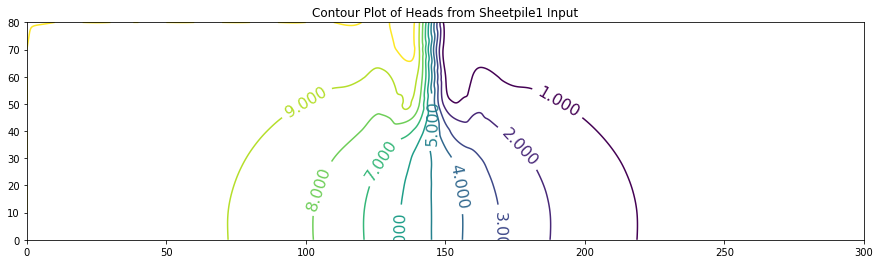
ax.set_title('Contour Plot of Heads from Sheetpile1 Input')
Exit iterations in velocity potential because tolerance met
Iterations = 443
End Calculations
Iterations    =  443
Closure Error =  0.0
Head Map
----
0 [10.    10.    10.    10.    10.    10.    10.    10.    10.    10.
 10.    10.    10.    10.     9.478  0.524  0.     0.     0.     0.
  0.     0.     0.     0.     0.     0.     0.     0.     0.     0.
  0.   ]
1 [10.     9.98   9.959  9.936  9.91   9.881  9.848  9.808  9.763  9.71
  9.652  9.591  9.535  9.497  9.478  0.524  0.505  0.467  0.411  0.351
  0.293  0.241  0.196  0.157  0.125  0.097  0.073  0.052  0.034  0.016
  0.   ]
2 [10.     9.96   9.919  9.874  9.824  9.767  9.701  9.623  9.532  9.426
  9.306  9.178  9.054  8.965  8.949  1.055  1.039  0.95   0.827  0.699
  0.58   0.475  0.385  0.309  0.244  0.19   0.143  0.102  0.066  0.032
  0.   ]
3 [10.     9.943  9.883  9.818  9.746  9.663  9.566  9.451  9.316  9.156
  8.969  8.759  8.538  8.351  8.336  1.67   1.654  1.468  1.247  1.038
  0.852  0.694  0.56   0.448  0.354  0.275  0.207  0.148  0.095  0.047
  0.   ]
4 [10.     9.927  9.852  9.77   9.678  9.572  9.448  9.3    9.124  8.912
  8.657  8.351  7.986  7.559  6.629  3.379  2.448  2.021  1.657  1.352
  1.098  0.888  0.714  0.57   0.45   0.348  0.262  0.187  0.121  0.059
  0.   ]
5 [10.     9.915  9.827  9.731  9.623  9.499  9.353  9.179  8.968  8.711
  8.395  8.002  7.498  6.806  5.702  4.307  3.202  2.511  2.007  1.615
  1.301  1.046  0.838  0.667  0.526  0.407  0.306  0.219  0.141  0.069
  0.   ]
6 [10.     9.907  9.81   9.704  9.586  9.448  9.287  9.093  8.858  8.569
  8.212  7.764  7.196  6.465  5.528  4.48   3.544  2.813  2.246  1.8
  1.444  1.158  0.926  0.736  0.579  0.448  0.337  0.24   0.155  0.076
  0.   ]
7 [10.     9.903  9.801  9.69   9.566  9.422  9.253  9.049  8.801  8.496
  8.118  7.647  7.057  6.33   5.467  4.542  3.679  2.952  2.364  1.894
  1.518  1.215  0.971  0.771  0.606  0.469  0.352  0.251  0.162  0.079
  0.   ]
8 [10.     9.903  9.801  9.69   9.566  9.422  9.253  9.049  8.801  8.496
  8.118  7.647  7.057  6.33   5.467  4.542  3.679  2.952  2.364  1.894
  1.518  1.215  0.971  0.771  0.606  0.469  0.352  0.251  0.162  0.079
  0.   ]
----
Text(0.5, 1.0, 'Contour Plot of Heads from Sheetpile1 Input')
Now we reuse the code, but change head to stream and modify the contour plot variable names as well as modify the input file to reflect the changed material properties and boundary conditions.
Here’s the input file for the stream function
10
10
1
9
31
1e-12
5000
0 10 20 30 40 50 60 70 80 90 100 110 120 130 140 150 160 170 180 190 200 210 220 230 240 250 260 270 280 290 300
80 70 60 50 40 30 20 10 0
0 0 0 0 0 0 0 0 0 0 0 0 0 0 1 1 0 0 0 0 0 0 0 0 0 0 0 0 0 0 0
1 1 1 1 1 1 1 1 1 1 1 1 1 1 1 1 1 1 1 1 1 1 1 1 1 1 1 1 1 1 1
1 1 1 1 1 1 1 1 1
1 1 1 1 1 1 1 1 1
100 0 0 0 0 0 0 0 0 0 0 0 0 0 0 0 0 0 0 0 0 0 0 0 0 0 0 0 0 0 100
100 0 0 0 0 0 0 0 0 0 0 0 0 0 0 0 0 0 0 0 0 0 0 0 0 0 0 0 0 0 100
100 0 0 0 0 0 0 0 0 0 0 0 0 0 0 0 0 0 0 0 0 0 0 0 0 0 0 0 0 0 100
100 0 0 0 0 0 0 0 0 0 0 0 0 0 0 0 0 0 0 0 0 0 0 0 0 0 0 0 0 0 100
100 0 0 0 0 0 0 0 0 0 0 0 0 0 0 0 0 0 0 0 0 0 0 0 0 0 0 0 0 0 100
100 0 0 0 0 0 0 0 0 0 0 0 0 0 0 0 0 0 0 0 0 0 0 0 0 0 0 0 0 0 100
100 0 0 0 0 0 0 0 0 0 0 0 0 0 0 0 0 0 0 0 0 0 0 0 0 0 0 0 0 0 100
100 0 0 0 0 0 0 0 0 0 0 0 0 0 0 0 0 0 0 0 0 0 0 0 0 0 0 0 0 0 100
100 100 100 100 100 100 100 100 100 100 100 100 100 100 100 100 100 100 100 100 100 100 100 100 100 100 100 100 100 100 100
10000 10000 10000 10000 10000 10000 10000 10000 10000 10000 10000 10000 10000 10000 10000000 10000000 10000 10000 10000 10000 10000 10000 10000 10000 10000 10000 10000 10000 10000 10000 10000
10000 10000 10000 10000 10000 10000 10000 10000 10000 10000 10000 10000 10000 10000 10000000 10000000 10000 10000 10000 10000 10000 10000 10000 10000 10000 10000 10000 10000 10000 10000 10000
10000 10000 10000 10000 10000 10000 10000 10000 10000 10000 10000 10000 10000 10000 10000000 10000000 10000 10000 10000 10000 10000 10000 10000 10000 10000 10000 10000 10000 10000 10000 10000
10000 10000 10000 10000 10000 10000 10000 10000 10000 10000 10000 10000 10000 10000 10000000 10000000 10000 10000 10000 10000 10000 10000 10000 10000 10000 10000 10000 10000 10000 10000 10000
10000 10000 10000 10000 10000 10000 10000 10000 10000 10000 10000 10000 10000 10000 10000000 10000000 10000 10000 10000 10000 10000 10000 10000 10000 10000 10000 10000 10000 10000 10000 10000
10000 10000 10000 10000 10000 10000 10000 10000 10000 10000 10000 10000 10000 10000 10000 10000 10000 10000 10000 10000 10000 10000 10000 10000 10000 10000 10000 10000 10000 10000 10000
10000 10000 10000 10000 10000 10000 10000 10000 10000 10000 10000 10000 10000 10000 10000 10000 10000 10000 10000 10000 10000 10000 10000 10000 10000 10000 10000 10000 10000 10000 10000
10000 10000 10000 10000 10000 10000 10000 10000 10000 10000 10000 10000 10000 10000 10000 10000 10000 10000 10000 10000 10000 10000 10000 10000 10000 10000 10000 10000 10000 10000 10000
10000 10000 10000 10000 10000 10000 10000 10000 10000 10000 10000 10000 10000 10000 10000 10000 10000 10000 10000 10000 10000 10000 10000 10000 10000 10000 10000 10000 10000 10000 100000
10000 10000 10000 10000 10000 10000 10000 10000 10000 10000 10000 10000 10000 10000 10000000 10000000 10000 10000 10000 10000 10000 10000 10000 10000 10000 10000 10000 10000 10000 10000 10000
10000 10000 10000 10000 10000 10000 10000 10000 10000 10000 10000 10000 10000 10000 10000000 10000000 10000 10000 10000 10000 10000 10000 10000 10000 10000 10000 10000 10000 10000 10000 10000
10000 10000 10000 10000 10000 10000 10000 10000 10000 10000 10000 10000 10000 10000 10000000 10000000 10000 10000 10000 10000 10000 10000 10000 10000 10000 10000 10000 10000 10000 10000 10000
10000 10000 10000 10000 10000 10000 10000 10000 10000 10000 10000 10000 10000 10000 10000000 10000000 10000 10000 10000 10000 10000 10000 10000 10000 10000 10000 10000 10000 10000 10000 10000
10000 10000 10000 10000 10000 10000 10000 10000 10000 10000 10000 10000 10000 10000 10000000 10000000 10000 10000 10000 10000 10000 10000 10000 10000 10000 10000 10000 10000 10000 10000 10000
10000 10000 10000 10000 10000 10000 10000 10000 10000 10000 10000 10000 10000 10000 10000 10000 10000 10000 10000 10000 10000 10000 10000 10000 10000 10000 10000 10000 10000 10000 10000
10000 10000 10000 10000 10000 10000 10000 10000 10000 10000 10000 10000 10000 10000 10000 10000 10000 10000 10000 10000 10000 10000 10000 10000 10000 10000 10000 10000 10000 10000 10000
10000 10000 10000 10000 10000 10000 10000 10000 10000 10000 10000 10000 10000 10000 10000 10000 10000 10000 10000 10000 10000 10000 10000 10000 10000 10000 10000 10000 10000 10000 10000
10000 10000 10000 10000 10000 10000 10000 10000 10000 10000 10000 10000 10000 10000 10000 10000 10000 10000 10000 10000 10000 10000 10000 10000 10000 10000 10000 10000 10000 10000 10000
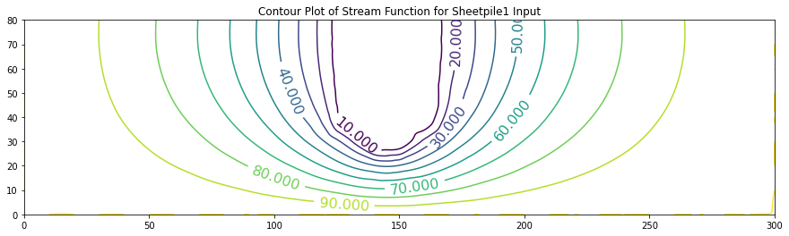
In these examples the value of the stream function is arbitrarily set to range from \(0\) to \(100\). One useful interpretation of stream function values is that their differences indicate the flow fraction (of total flow) that flows between the streamlines (contour lines of constant stream function value).
def sse(matrix1,matrix2):
    sse=0.0
    nr=len(matrix1) # get row count
    nc=len(matrix1[0]) # get column count
    for ir in range(nr):
        for jc in range(nc):
            sse=sse+(matrix1[ir][jc]-matrix2[ir][jc])**2
    return(sse)

def update(matrix1,matrix2):
    nr=len(matrix1) # get row count
    nc=len(matrix1[0]) # get column count
    ##print(nr,nc)
    for ir in range(nr):
        for jc in range(nc):
            ##print(ir,jc)
            matrix2[ir][jc]=matrix1[ir][jc]
    return(matrix2)

def writearray(matrix):
    nr=len(matrix) # get row count
    nc=len(matrix[0]) # get column count
    import numpy as np
    new_list = list(np.around(np.array(matrix), 3))
    for ir in range(nr):
        print(ir,new_list[ir][:])
    return()

localfile = open("StreamFnSheetpile1.txt","r") # connect and read file for 2D gw model
deltax = float(localfile.readline())
deltay = float(localfile.readline())
deltaz = float(localfile.readline())
nrows = int(localfile.readline())
ncols = int(localfile.readline())
tolerance = float(localfile.readline())
maxiter = int(localfile.readline())
distancex = [] # empty list
distancex.append([float(n) for n in localfile.readline().strip().split()])
distancey = [] # empty list
distancey.append([float(n) for n in localfile.readline().strip().split()])
boundarytop = [] #empty list
boundarytop.append([float(n) for n in localfile.readline().strip().split()])
boundarybottom = [] #empty list
boundarybottom.append([int(n) for n in localfile.readline().strip().split()])
boundaryleft = [] #empty list
boundaryleft.append([int(n) for n in localfile.readline().strip().split()])
boundaryright = [] #empty list
boundaryright.append([int(n) for n in localfile.readline().strip().split()])
stream =[] # empty list
for irow in range(nrows):
        stream.append([float(n) for n in localfile.readline().strip().split()])
hydcondx = [] # empty list
for irow in range(nrows):
        hydcondx.append([float(n) for n in localfile.readline().strip().split()])
hydcondy = [] # empty list
for irow in range(nrows):
        hydcondy.append([float(n) for n in localfile.readline().strip().split()])
localfile.close() # Disconnect the file
##
amat = [[0 for j in range(ncols)] for i in range(nrows)]
bmat = [[0 for j in range(ncols)] for i in range(nrows)]
cmat = [[0 for j in range(ncols)] for i in range(nrows)]
dmat = [[0 for j in range(ncols)] for i in range(nrows)]
##
for irow in range(1,nrows-1):
    for jcol in range(1,ncols-1):
        amat[irow][jcol] = (( hydcondx[irow-1][jcol  ]+ hydcondx[irow  ][jcol  ]) * deltaz ) /(2.0*deltax**2)
        bmat[irow][jcol] = (( hydcondx[irow  ][jcol  ]+ hydcondx[irow+1][jcol  ]) * deltaz ) /(2.0*deltax**2)
        cmat[irow][jcol] = (( hydcondy[irow  ][jcol-1]+ hydcondy[irow  ][jcol  ]) * deltaz ) /(2.0*deltay**2)
        dmat[irow][jcol] = (( hydcondy[irow  ][jcol  ]+ hydcondy[irow  ][jcol+1]) * deltaz ) /(2.0*deltay**2)
##
streamold = [[0 for jc in range(ncols)] for ir in range(nrows)] #force new matrix
streamold = update(stream,streamold) # update
##writearray(stream)
##print("----")
##writearray(streamold)
##print("--------")
tolflag = False
for iter in range(maxiter):
##    print("begin iteration")
##    writearray(stream)
##    print("----")
##    writearray(streamold)
##    print("--------")

# Boundary Conditions

# first and last row special == no flow boundaries
    for jcol in range(ncols):
        if boundarytop[0][jcol] == 0: # no - flow at top
            stream [0][jcol ] = stream[1][jcol ]
        if boundarybottom[0][ jcol ] == 0: # no - flow at bottom
            stream [nrows-1][jcol ] = stream[nrows-2][jcol ]
# first and last column special == no flow boundaries
    for irow in range(nrows):
        if  boundaryleft[0][ irow ] == 0:
            stream[irow][0] = stream [irow][1] # no - flow at left
        if boundaryright[0][ irow ] == 0:
            stream [irow][ncols-1] = stream[ irow ][ncols-2] # no - flow at right
# interior updates
    for irow in range(1,nrows-1):
        for jcol in range(1,ncols-1):
            stream[irow][jcol]=( amat[irow][jcol]*stream[irow-1][jcol  ]
                              +bmat[irow][jcol]*stream[irow+1][jcol  ]
                              +cmat[irow][jcol]*stream[irow  ][jcol-1]
                              +dmat[irow][jcol]*stream[irow  ][jcol+1])/(amat[ irow][jcol ]+ bmat[ irow][jcol ]+ cmat[ irow][jcol ]+ dmat[ irow][jcol ])
# test for stopping iterations
##    print("end iteration")
##    writearray(stream)
##    print("----")
##    writearray(streamold)
    percentdiff = sse(stream,streamold)
    if  percentdiff <= tolerance:
        print("Exit iterations in Stream Function because tolerance met ")
        print("Iterations =" , iter+1 ) ;
        tolflag = True
        break
    streamold = update(stream,streamold)
print("End Calculations")
print("Iterations    = ",iter+1)
print("Closure Error = ",round(percentdiff,3))
print("Stream Function Map")
print("----")
writearray(stream)
print("----")
####################### Contour Plot ###############
my_xyz2 = [] # empty list
for irow in range(nrows):
    for jcol in range(ncols):
        my_xyz2.append([distancex[0][jcol],distancey[0][irow],stream[irow][jcol]])
import pandas
my_xyz2 = pandas.DataFrame(my_xyz2) # convert into a data frame
#print(my_xyz) # activate to examine the dataframe
import numpy
import matplotlib.pyplot
from scipy.interpolate import griddata
# extract lists from the dataframe
coord_x2 = my_xyz2[0].values.tolist() # column 0 of dataframe
coord_y2 = my_xyz2[1].values.tolist() # column 1 of dataframe
coord_z2 = my_xyz2[2].values.tolist() # column 2 of dataframe
coord_xy2 = numpy.column_stack((coord_x2, coord_y2))
# Set plotting range in original data units
lon = numpy.linspace(min(coord_x2), max(coord_x2), 3000)
lat = numpy.linspace(min(coord_y2), max(coord_y2), 800)
X2, Y2 = numpy.meshgrid(lon, lat)
# Grid the data; use linear interpolation (choices are nearest, linear, cubic)
Z2 = griddata(numpy.array(coord_xy2), numpy.array(coord_z2), (X2, Y2), method='cubic')
# Build the map
fig, ax = matplotlib.pyplot.subplots()
fig.set_size_inches(15, 4)
levels = [10,20,30,40,50,60,70,80,90,100]
CS2 = ax.contour(X2, Y2, Z2, levels )
ax.clabel(CS2, inline=2, fontsize=16)
ax.set_title('Contour Plot of Stream Function for Sheetpile1 Input')
Exit iterations in Stream Function because tolerance met
Iterations = 396
End Calculations
Iterations    =  396
Closure Error =  0.0
Stream Function Map
----
0 [100.     96.845  93.555  89.987  85.989  81.394  76.015  69.642  62.046
  52.99   42.26   29.74   15.542   0.191   0.      0.      0.19   15.469
  29.592  42.031  52.669  61.62   69.093  75.318  80.519  84.898  88.632
  91.878  94.773  97.442 100.   ]
1 [100.     96.845  93.555  89.987  85.989  81.394  76.015  69.642  62.046
  52.99   42.26   29.74   15.542   0.191   0.16    0.16    0.19   15.469
  29.592  42.031  52.669  61.62   69.093  75.318  80.519  84.898  88.632
  91.878  94.773  97.442 100.   ]
2 [100.     96.982  93.832  90.416  86.586  82.178  77.008  70.865  63.507
  54.663  44.05   31.419  16.694   0.337   0.304   0.304   0.336  16.625
  31.277  43.83   54.356  63.099  70.34   76.342  81.342  85.543  89.121
  92.229  94.999  97.553 100.   ]
3 [100.     97.249  94.377  91.26   87.76   83.724  78.976  73.304  66.452
  58.105  47.859  35.19   19.48    0.47    0.432   0.432   0.47   19.416
  35.061  47.658  57.826  66.081  72.825  78.369  82.963  86.81   90.08
  92.916  95.443  97.77  100.   ]
4 [100.     97.636  95.168  92.486  89.47   85.984  81.867  76.921  70.894
  63.447  54.089  42.004  25.566   0.634   0.541   0.541   0.634  25.509
  41.891  53.916  63.207  70.575  76.51   81.346  85.33   88.655  91.473
  93.914  96.085  98.085 100.   ]
5 [100.     98.128  96.172  94.045  91.65   88.875  85.587  81.619  76.754
  70.701  63.045  53.171  40.146  22.721   0.665   0.665  22.703  40.095
  53.079  62.907  70.511  76.502  81.294  85.175  88.358  91.005  93.244
  95.18   96.901  98.484 100.   ]
6 [100.     98.703  97.348  95.872  94.209  92.279  89.987  87.213  83.804
  79.559  74.22   67.487  59.128  49.437  40.688  40.683  49.419  59.09
  67.422  74.124  79.426  83.629  86.988  89.702  91.921  93.763  95.318
  96.661  97.853  98.95  100.   ]
7 [100.     99.336  98.643  97.888  97.036  96.046  94.869  93.443  91.689
  89.509  86.79   83.43   79.442  75.211  71.965  71.962  75.201  79.422
  83.396  86.74   89.442  91.6    93.328  94.723  95.863  96.808  97.604
  98.292  98.902  99.463 100.   ]
8 [100. 100. 100. 100. 100. 100. 100. 100. 100. 100. 100. 100. 100. 100.
 100. 100. 100. 100. 100. 100. 100. 100. 100. 100. 100. 100. 100. 100.
 100. 100. 100.]
----
Text(0.5, 1.0, 'Contour Plot of Stream Function for Sheetpile1 Input')
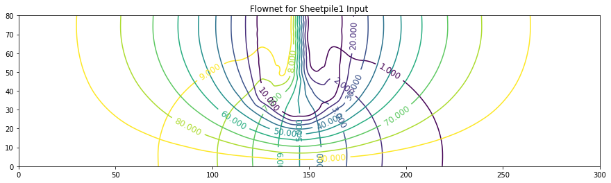
Now both plots on same canvass
# Head (Velocity Potential Map)
# Grid the data; use linear interpolation (choices are nearest, linear, cubic)
Z = griddata(numpy.array(coord_xy), numpy.array(coord_z), (X, Y), method='cubic')
Z2 = griddata(numpy.array(coord_xy2), numpy.array(coord_z2), (X2, Y2), method='cubic')
# Build the map
fig, ax = matplotlib.pyplot.subplots()
fig.set_size_inches(15, 4)
levels1 = [1,2,3,4,5,6,7,8,9]
CS = ax.contour(X, Y, Z, levels1)
levels2 = [10,20,30,40,50,60,70,80,90]
CS2 = ax.contour(X2, Y2, Z2, levels2 )
ax.clabel(CS, inline=2, fontsize=12)
ax.clabel(CS2, inline=2, fontsize=12)
ax.set_title('Flownet for Sheetpile1 Input')
Text(0.5, 1.0, 'Flownet for Sheetpile1 Input')
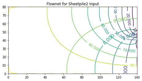
Flownet Example 2 : Pore Pressure under a Dam (Domain Decomposition approach)
The second way to solve this example, and perhaps better is to take advantage of the symmetry and cut the domain in half, as

In this method we can actually specify the sheetpile as a boundary, and we will obtain the about same results, but only need to supply half as much input data.
Here’s the input file for the half-domain head calculations
10
10
1
9
15
1e-16
5000
0 10 20 30 40 50 60 70 80 90 100 110 120 130 140
80 70 60 50 40 30 20 10 0
1 1 1 1 1 1 1 1 1 1 1 1 1 1 1
0 0 0 0 0 0 0 0 0 0 0 0 0 0 0
1 1 1 1 1 1 1 1 1
0 0 0 0 1 1 1 1 1
10 10 10 10 10 10 10 10 10 10 10 10 10 10 10
10 10 10 10 10 10 10 10 10 10 10 10 10 10 10
10 10 10 10 10 10 10 10 10 10 10 10 10 10 10
10 10 10 10 10 10 10 10 10 10 10 10 10 10 10
10 10 10 10 10 10 10 10 10 10 10 10 10 10 5
10 10 10 10 10 10 10 10 10 10 10 10 10 10 5
10 10 10 10 10 10 10 10 10 10 10 10 10 10 5
10 10 10 10 10 10 10 10 10 10 10 10 10 10 5
10 10 10 10 10 10 10 10 10 10 10 10 10 10 5
0.0001 0.0001 0.0001 0.0001 0.0001 0.0001 0.0001 0.0001 0.0001 0.0001 0.0001 0.0001 0.0001 0.0001 0.0001
0.0001 0.0001 0.0001 0.0001 0.0001 0.0001 0.0001 0.0001 0.0001 0.0001 0.0001 0.0001 0.0001 0.0001 0.0001
0.0001 0.0001 0.0001 0.0001 0.0001 0.0001 0.0001 0.0001 0.0001 0.0001 0.0001 0.0001 0.0001 0.0001 0.0001
0.0001 0.0001 0.0001 0.0001 0.0001 0.0001 0.0001 0.0001 0.0001 0.0001 0.0001 0.0001 0.0001 0.0001 0.0001
0.0001 0.0001 0.0001 0.0001 0.0001 0.0001 0.0001 0.0001 0.0001 0.0001 0.0001 0.0001 0.0001 0.0001 0.0001
0.0001 0.0001 0.0001 0.0001 0.0001 0.0001 0.0001 0.0001 0.0001 0.0001 0.0001 0.0001 0.0001 0.0001 0.0001
0.0001 0.0001 0.0001 0.0001 0.0001 0.0001 0.0001 0.0001 0.0001 0.0001 0.0001 0.0001 0.0001 0.0001 0.0001
0.0001 0.0001 0.0001 0.0001 0.0001 0.0001 0.0001 0.0001 0.0001 0.0001 0.0001 0.0001 0.0001 0.0001 0.0001
0.0001 0.0001 0.0001 0.0001 0.0001 0.0001 0.0001 0.0001 0.0001 0.0001 0.0001 0.0001 0.0001 0.0001 0.0001
0.0001 0.0001 0.0001 0.0001 0.0001 0.0001 0.0001 0.0001 0.0001 0.0001 0.0001 0.0001 0.0001 0.0001 0.0001
0.0001 0.0001 0.0001 0.0001 0.0001 0.0001 0.0001 0.0001 0.0001 0.0001 0.0001 0.0001 0.0001 0.0001 0.0001
0.0001 0.0001 0.0001 0.0001 0.0001 0.0001 0.0001 0.0001 0.0001 0.0001 0.0001 0.0001 0.0001 0.0001 0.0001
0.0001 0.0001 0.0001 0.0001 0.0001 0.0001 0.0001 0.0001 0.0001 0.0001 0.0001 0.0001 0.0001 0.0001 0.0001
0.0001 0.0001 0.0001 0.0001 0.0001 0.0001 0.0001 0.0001 0.0001 0.0001 0.0001 0.0001 0.0001 0.0001 0.0001
0.0001 0.0001 0.0001 0.0001 0.0001 0.0001 0.0001 0.0001 0.0001 0.0001 0.0001 0.0001 0.0001 0.0001 0.0001
0.0001 0.0001 0.0001 0.0001 0.0001 0.0001 0.0001 0.0001 0.0001 0.0001 0.0001 0.0001 0.0001 0.0001 0.0001
0.0001 0.0001 0.0001 0.0001 0.0001 0.0001 0.0001 0.0001 0.0001 0.0001 0.0001 0.0001 0.0001 0.0001 0.0001
0.0001 0.0001 0.0001 0.0001 0.0001 0.0001 0.0001 0.0001 0.0001 0.0001 0.0001 0.0001 0.0001 0.0001 0.0001
def sse(matrix1,matrix2):
sse=0.0
nr=len(matrix1) # get row count
nc=len(matrix1[0]) # get column count
for ir in range(nr):
for jc in range(nc):
sse=sse+(matrix1[ir][jc]-matrix2[ir][jc])**2
return(sse)
def update(matrix1,matrix2):
nr=len(matrix1) # get row count
nc=len(matrix1[0]) # get column count
##print(nr,nc)
for ir in range(nr):
for jc in range(nc):
##print(ir,jc)
matrix2[ir][jc]=matrix1[ir][jc]
return(matrix2)
def writearray(matrix):
nr=len(matrix) # get row count
nc=len(matrix[0]) # get column count
import numpy as np
new_list = list(np.around(np.array(matrix), 3))
for ir in range(nr):
print(ir,new_list[ir][:])
return()
localfile = open("PotentialFnSheetpile2.txt","r") # connect and read file for 2D gw model
deltax = float(localfile.readline())
deltay = float(localfile.readline())
deltaz = float(localfile.readline())
nrows = int(localfile.readline())
ncols = int(localfile.readline())
tolerance = float(localfile.readline())
maxiter = int(localfile.readline())
distancex = [] # empty list
distancex.append([float(n) for n in localfile.readline().strip().split()])
distancey = [] # empty list
distancey.append([float(n) for n in localfile.readline().strip().split()])
boundarytop = [] #empty list
boundarytop.append([float(n) for n in localfile.readline().strip().split()])
boundarybottom = [] #empty list
boundarybottom.append([int(n) for n in localfile.readline().strip().split()])
boundaryleft = [] #empty list
boundaryleft.append([int(n) for n in localfile.readline().strip().split()])
boundaryright = [] #empty list
boundaryright.append([int(n) for n in localfile.readline().strip().split()])
head =[] # empty list
for irow in range(nrows):
head.append([float(n) for n in localfile.readline().strip().split()])
hydcondx = [] # empty list
for irow in range(nrows):
hydcondx.append([float(n) for n in localfile.readline().strip().split()])
hydcondy = [] # empty list
for irow in range(nrows):
hydcondy.append([float(n) for n in localfile.readline().strip().split()])
localfile.close() # Disconnect the file
##
amat = [[0 for j in range(ncols)] for i in range(nrows)]
bmat = [[0 for j in range(ncols)] for i in range(nrows)]
cmat = [[0 for j in range(ncols)] for i in range(nrows)]
dmat = [[0 for j in range(ncols)] for i in range(nrows)]
##
for irow in range(1,nrows-1):
for jcol in range(1,ncols-1):
amat[irow][jcol] = (( hydcondx[irow-1][jcol ]+ hydcondx[irow ][jcol ]) * deltaz ) /(2.0*deltax**2)
bmat[irow][jcol] = (( hydcondx[irow ][jcol ]+ hydcondx[irow+1][jcol ]) * deltaz ) /(2.0*deltax**2)
cmat[irow][jcol] = (( hydcondy[irow ][jcol-1]+ hydcondy[irow ][jcol ]) * deltaz ) /(2.0*deltay**2)
dmat[irow][jcol] = (( hydcondy[irow ][jcol ]+ hydcondy[irow ][jcol+1]) * deltaz ) /(2.0*deltay**2)
##
headold = [[0 for jc in range(ncols)] for ir in range(nrows)] #force new matrix
headold = update(head,headold) # update
##writearray(head)
##print("----")
##writearray(headold)
##print("--------")
tolflag = False
for iter in range(maxiter):
## print("begin iteration")
## writearray(head)
## print("----")
## writearray(headold)
## print("--------")
# Boundary Conditions
# first and last row special == no flow boundaries
for jcol in range(ncols):
if boundarytop[0][jcol] == 0: # no - flow at top
head [0][jcol ] = head[1][jcol ]
if boundarybottom[0][ jcol ] == 0: # no - flow at bottom
head [nrows-1][jcol ] = head[nrows-2][jcol ]
# first and last column special == no flow boundaries
for irow in range(nrows):
if boundaryleft[0][ irow ] == 0:
head[irow][0] = head [irow][1] # no - flow at left
if boundaryright[0][ irow ] == 0:
head [irow][ncols-1] = head[ irow ][ncols-2] # no - flow at right
# interior updates
for irow in range(1,nrows-1):
for jcol in range(1,ncols-1):
head[irow][jcol]=( amat[irow][jcol]*head[irow-1][jcol ]
+bmat[irow][jcol]*head[irow+1][jcol ]
+cmat[irow][jcol]*head[irow ][jcol-1]
+dmat[irow][jcol]*head[irow ][jcol+1])/(amat[ irow][jcol ]+ bmat[ irow][jcol ]+ cmat[ irow][jcol ]+ dmat[ irow][jcol ])
# test for stopping iterations
## print("end iteration")
## writearray(head)
## print("----")
## writearray(headold)
percentdiff = sse(head,headold)
if percentdiff <= tolerance:
print("Exit iterations in velocity potential because tolerance met ")
print("Iterations =" , iter+1 ) ;
tolflag = True
break
headold = update(head,headold)
print("End Calculations")
print("Iterations = ",iter+1)
print("Closure Error = ",round(percentdiff,3))
print("Head Map")
print("----")
writearray(head)
print("----")
############# Contour Plot
my_xyz = [] # empty list
for irow in range(nrows):
for jcol in range(ncols):
my_xyz.append([distancex[0][jcol],distancey[0][irow],head[irow][jcol]])
import pandas
my_xyz = pandas.DataFrame(my_xyz) # convert into a data frame
#print(my_xyz) # activate to examine the dataframe
import numpy
import matplotlib.pyplot
from scipy.interpolate import griddata
# extract lists from the dataframe
coord_x = my_xyz[0].values.tolist() # column 0 of dataframe
coord_y = my_xyz[1].values.tolist() # column 1 of dataframe
coord_z = my_xyz[2].values.tolist() # column 2 of dataframe
coord_xy = numpy.column_stack((coord_x, coord_y))
# Set plotting range in original data units
lon = numpy.linspace(min(coord_x), max(coord_x), 3000)
lat = numpy.linspace(min(coord_y), max(coord_y), 800)
X, Y = numpy.meshgrid(lon, lat)
# Grid the data; use linear interpolation (choices are nearest, linear, cubic)
Z = griddata(numpy.array(coord_xy), numpy.array(coord_z), (X, Y), method='cubic')
# Build the map
fig, ax = matplotlib.pyplot.subplots()
fig.set_size_inches(7.5, 4)
levels1 = [1,2,3,4,5,6,7,8,9,10]
CS = ax.contour(X, Y, Z, levels1)
ax.clabel(CS, inline=2, fontsize=16)
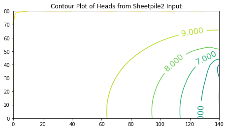
ax.set_title('Contour Plot of Heads from Sheetpile2 Input')
Exit iterations in velocity potential because tolerance met
Iterations = 412
End Calculations
Iterations    =  412
Closure Error =  0.0
Head Map
----
0 [10. 10. 10. 10. 10. 10. 10. 10. 10. 10. 10. 10. 10. 10. 10.]
1 [10.     9.975  9.949  9.921  9.889  9.853  9.811  9.761  9.701  9.632
  9.552  9.466  9.384  9.329  9.329]
2 [10.     9.951  9.9    9.845  9.783  9.712  9.629  9.531  9.413  9.274
  9.111  8.928  8.742  8.602  8.602]
3 [10.     9.93   9.856  9.776  9.687  9.584  9.463  9.319  9.147  8.939
  8.69   8.393  8.056  7.734  7.734]
4 [10.     9.911  9.818  9.717  9.604  9.473  9.32   9.137  8.916  8.647
  8.316  7.9    7.353  6.544  5.   ]
5 [10.     9.896  9.788  9.67   9.538  9.385  9.206  8.992  8.733  8.416
  8.026  7.538  6.913  6.088  5.   ]
6 [10.     9.886  9.767  9.637  9.492  9.325  9.127  8.891  8.607  8.26
  7.835  7.313  6.672  5.895  5.   ]
7 [10.     9.881  9.756  9.621  9.469  9.293  9.087  8.84   8.543  8.181
  7.741  7.207  6.566  5.82   5.   ]
8 [10.     9.881  9.756  9.621  9.469  9.293  9.087  8.84   8.543  8.181
  7.741  7.207  6.566  5.82   5.   ]
----
Text(0.5, 1.0, 'Contour Plot of Heads from Sheetpile2 Input')
Note
If you have to do this a lot, you could automate the “file rewrite” and have the program run the two instances back to back then make the contour plots
Here’s the input file for the domain decomposition stream function calculations
10
10
1
9
15
1e-16
5000
0 10 20 30 40 50 60 70 80 90 100 110 120 130 140
80 70 60 50 40 30 20 10 0
1 0 0 0 0 0 0 0 0 0 0 0 0 0 1
1 1 1 1 1 1 1 1 1 1 1 1 1 1 1
1 1 1 1 1 1 1 1 1
1 1 1 1 0 0 0 0 0
100 5 5 5 5 5 5 5 5 5 5 5 5 5 0
100 5 5 5 5 5 5 5 5 5 5 5 5 5 0
100 5 5 5 5 5 5 5 5 5 5 5 5 5 0
100 5 5 5 5 5 5 5 5 5 5 5 5 5 0
100 5 5 5 5 5 5 5 5 5 5 5 5 5 0
100 5 5 5 5 5 5 5 5 5 5 5 5 5 0
100 5 5 5 5 5 5 5 5 5 5 5 5 5 0
100 5 5 5 5 5 5 5 5 5 5 5 5 5 0
100 100 100 100 100 100 100 100 100 100 100 100 100 100 100
100000 100000 100000 100000 100000 100000 100000 100000 100000 100000 100000 100000 100000 100000 100000
100000 100000 100000 100000 100000 100000 100000 100000 100000 100000 100000 100000 100000 100000 100000
100000 100000 100000 100000 100000 100000 100000 100000 100000 100000 100000 100000 100000 100000 100000
100000 100000 100000 100000 100000 100000 100000 100000 100000 100000 100000 100000 100000 100000 100000
100000 100000 100000 100000 100000 100000 100000 100000 100000 100000 100000 100000 100000 100000 100000
100000 100000 100000 100000 100000 100000 100000 100000 100000 100000 100000 100000 100000 100000 100000
100000 100000 100000 100000 100000 100000 100000 100000 100000 100000 100000 100000 100000 100000 100000
100000 100000 100000 100000 100000 100000 100000 100000 100000 100000 100000 100000 100000 100000 100000
100000 100000 100000 100000 100000 100000 100000 100000 100000 100000 100000 100000 100000 100000 100000
100000 100000 100000 100000 100000 100000 100000 100000 100000 100000 100000 100000 100000 100000 100000
100000 100000 100000 100000 100000 100000 100000 100000 100000 100000 100000 100000 100000 100000 100000
100000 100000 100000 100000 100000 100000 100000 100000 100000 100000 100000 100000 100000 100000 100000
100000 100000 100000 100000 100000 100000 100000 100000 100000 100000 100000 100000 100000 100000 100000
100000 100000 100000 100000 100000 100000 100000 100000 100000 100000 100000 100000 100000 100000 100000
100000 100000 100000 100000 100000 100000 100000 100000 100000 100000 100000 100000 100000 100000 100000
100000 100000 100000 100000 100000 100000 100000 100000 100000 100000 100000 100000 100000 100000 100000
100000 100000 100000 100000 100000 100000 100000 100000 100000 100000 100000 100000 100000 100000 100000
100000 100000 100000 100000 100000 100000 100000 100000 100000 100000 100000 100000 100000 100000 100000
def sse(matrix1,matrix2):
    sse=0.0
    nr=len(matrix1) # get row count
    nc=len(matrix1[0]) # get column count
    for ir in range(nr):
        for jc in range(nc):
            sse=sse+(matrix1[ir][jc]-matrix2[ir][jc])**2
    return(sse)

def update(matrix1,matrix2):
    nr=len(matrix1) # get row count
    nc=len(matrix1[0]) # get column count
    ##print(nr,nc)
    for ir in range(nr):
        for jc in range(nc):
            ##print(ir,jc)
            matrix2[ir][jc]=matrix1[ir][jc]
    return(matrix2)

def writearray(matrix):
    nr=len(matrix) # get row count
    nc=len(matrix[0]) # get column count
    import numpy as np
    new_list = list(np.around(np.array(matrix), 3))
    for ir in range(nr):
        print(ir,new_list[ir][:])
    return()

localfile = open("StreamFnSheetpile2.txt","r") # connect and read file for 2D gw model
deltax = float(localfile.readline())
deltay = float(localfile.readline())
deltaz = float(localfile.readline())
nrows = int(localfile.readline())
ncols = int(localfile.readline())
tolerance = float(localfile.readline())
maxiter = int(localfile.readline())
distancex = [] # empty list
distancex.append([float(n) for n in localfile.readline().strip().split()])
distancey = [] # empty list
distancey.append([float(n) for n in localfile.readline().strip().split()])
boundarytop = [] #empty list
boundarytop.append([float(n) for n in localfile.readline().strip().split()])
boundarybottom = [] #empty list
boundarybottom.append([int(n) for n in localfile.readline().strip().split()])
boundaryleft = [] #empty list
boundaryleft.append([int(n) for n in localfile.readline().strip().split()])
boundaryright = [] #empty list
boundaryright.append([int(n) for n in localfile.readline().strip().split()])
stream =[] # empty list
for irow in range(nrows):
        stream.append([float(n) for n in localfile.readline().strip().split()])
hydcondx = [] # empty list
for irow in range(nrows):
        hydcondx.append([float(n) for n in localfile.readline().strip().split()])
hydcondy = [] # empty list
for irow in range(nrows):
        hydcondy.append([float(n) for n in localfile.readline().strip().split()])
localfile.close() # Disconnect the file
##
amat = [[0 for j in range(ncols)] for i in range(nrows)]
bmat = [[0 for j in range(ncols)] for i in range(nrows)]
cmat = [[0 for j in range(ncols)] for i in range(nrows)]
dmat = [[0 for j in range(ncols)] for i in range(nrows)]
##
for irow in range(1,nrows-1):
    for jcol in range(1,ncols-1):
        amat[irow][jcol] = (( hydcondx[irow-1][jcol  ]+ hydcondx[irow  ][jcol  ]) * deltaz ) /(2.0*deltax**2)
        bmat[irow][jcol] = (( hydcondx[irow  ][jcol  ]+ hydcondx[irow+1][jcol  ]) * deltaz ) /(2.0*deltax**2)
        cmat[irow][jcol] = (( hydcondy[irow  ][jcol-1]+ hydcondy[irow  ][jcol  ]) * deltaz ) /(2.0*deltay**2)
        dmat[irow][jcol] = (( hydcondy[irow  ][jcol  ]+ hydcondy[irow  ][jcol+1]) * deltaz ) /(2.0*deltay**2)
##
streamold = [[0 for jc in range(ncols)] for ir in range(nrows)] #force new matrix
streamold = update(stream,streamold) # update
##writearray(stream)
##print("----")
##writearray(streamold)
##print("--------")
tolflag = False
for iter in range(maxiter):
##    print("begin iteration")
##    writearray(stream)
##    print("----")
##    writearray(streamold)
##    print("--------")

# Boundary Conditions

# first and last row special == no flow boundaries
    for jcol in range(ncols):
        if boundarytop[0][jcol] == 0: # no - flow at top
            stream [0][jcol ] = stream[1][jcol ]
        if boundarybottom[0][ jcol ] == 0: # no - flow at bottom
            stream [nrows-1][jcol ] = stream[nrows-2][jcol ]
# first and last column special == no flow boundaries
    for irow in range(nrows):
        if  boundaryleft[0][ irow ] == 0:
            stream[irow][0] = stream [irow][1] # no - flow at left
        if boundaryright[0][ irow ] == 0:
            stream [irow][ncols-1] = stream[ irow ][ncols-2] # no - flow at right
# interior updates
    for irow in range(1,nrows-1):
        for jcol in range(1,ncols-1):
            stream[irow][jcol]=( amat[irow][jcol]*stream[irow-1][jcol  ]
                              +bmat[irow][jcol]*stream[irow+1][jcol  ]
                              +cmat[irow][jcol]*stream[irow  ][jcol-1]
                              +dmat[irow][jcol]*stream[irow  ][jcol+1])/(amat[ irow][jcol ]+ bmat[ irow][jcol ]+ cmat[ irow][jcol ]+ dmat[ irow][jcol ])
# test for stopping iterations
##    print("end iteration")
##    writearray(stream)
##    print("----")
##    writearray(streamold)
    percentdiff = sse(stream,streamold)
    if  percentdiff <= tolerance:
        print("Exit iterations in Stream Function because tolerance met ")
        print("Iterations =" , iter+1 ) ;
        tolflag = True
        break
    streamold = update(stream,streamold)
print("End Calculations")
print("Iterations    = ",iter+1)
print("Closure Error = ",round(percentdiff,3))
print("Stream Function Map")
print("----")
writearray(stream)
print("----")
####################### Contour Plot ###############
my_xyz2 = [] # empty list
for irow in range(nrows):
    for jcol in range(ncols):
        my_xyz2.append([distancex[0][jcol],distancey[0][irow],stream[irow][jcol]])
import pandas
my_xyz2 = pandas.DataFrame(my_xyz2) # convert into a data frame
#print(my_xyz) # activate to examine the dataframe
import numpy
import matplotlib.pyplot
from scipy.interpolate import griddata
# extract lists from the dataframe
coord_x2 = my_xyz2[0].values.tolist() # column 0 of dataframe
coord_y2 = my_xyz2[1].values.tolist() # column 1 of dataframe
coord_z2 = my_xyz2[2].values.tolist() # column 2 of dataframe
coord_xy2 = numpy.column_stack((coord_x2, coord_y2))
# Set plotting range in original data units
lon = numpy.linspace(min(coord_x2), max(coord_x2), 3000)
lat = numpy.linspace(min(coord_y2), max(coord_y2), 800)
X2, Y2 = numpy.meshgrid(lon, lat)
# Grid the data; use linear interpolation (choices are nearest, linear, cubic)
Z2 = griddata(numpy.array(coord_xy2), numpy.array(coord_z2), (X2, Y2), method='cubic')
# Build the map
fig, ax = matplotlib.pyplot.subplots()
fig.set_size_inches(7.5, 4)
levels = [5,20,30,40,50,60,70,80,90,100]
CS2 = ax.contour(X2, Y2, Z2, levels )
ax.clabel(CS2, inline=2, fontsize=16)
ax.set_title('Contour Plot of Stream Function for Sheetpile2 Input')
Exit iterations in Stream Function because tolerance met
Iterations = 523
End Calculations
Iterations    =  523
Closure Error =  0.0
Stream Function Map
----
0 [100.     97.905  95.718  93.34   90.663  87.566  83.901  79.49   74.106
  67.455  59.153  48.703  35.523  19.154   0.   ]
1 [100.     97.905  95.718  93.34   90.663  87.566  83.901  79.49   74.106
  67.455  59.153  48.703  35.523  19.154   0.   ]
2 [100.     97.998  95.909  93.638  91.084  88.133  84.648  80.463  75.373
  69.107  61.301  51.433  38.712  21.939   0.   ]
3 [100.     98.18   96.28   94.218  91.903  89.234  86.093  82.343  77.815
  72.298  65.51   57.018  45.952  29.889   0.   ]
4 [100.     98.441  96.815  95.051  93.076  90.806  88.149  85.001  81.245
  76.759  71.424  65.177  58.188  51.667  51.667]
5 [100.     98.769  97.486  96.097  94.544  92.766  90.696  88.265  85.406
  82.069  78.252  74.077  69.956  66.924  66.924]
6 [100.     99.15   98.264  97.305  96.237  95.017  93.604  91.958  90.046
  87.859  85.437  82.922  80.636  79.149  79.149]
7 [100.     99.566  99.114  98.625  98.081  97.461  96.745  95.916  94.962
  93.884  92.715  91.538  90.515  89.888  89.888]
8 [100. 100. 100. 100. 100. 100. 100. 100. 100. 100. 100. 100. 100. 100.
 100.]
----
Text(0.5, 1.0, 'Contour Plot of Stream Function for Sheetpile2 Input')
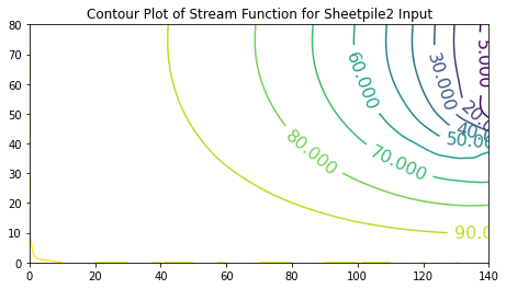
Now try both contour plot same plot canvas
# Head (Velocity Potential Map)
# Grid the data; use linear interpolation (choices are nearest, linear, cubic)
Z = griddata(numpy.array(coord_xy), numpy.array(coord_z), (X, Y), method='cubic')
Z2 = griddata(numpy.array(coord_xy2), numpy.array(coord_z2), (X2, Y2), method='cubic')
# Build the map
fig, ax = matplotlib.pyplot.subplots()
fig.set_size_inches(7.5, 4)
levels1 = [5,6,7,8,9,10]
CS = ax.contour(X, Y, Z, levels1)
levels2 = [10,20,30,40,50,60,70,80,90,100]
CS2 = ax.contour(X2, Y2, Z2, levels2 )
ax.clabel(CS, inline=2, fontsize=16)
ax.clabel(CS2, inline=2, fontsize=12)
ax.set_title('Flownet for Sheetpile2 Input')
Text(0.5, 1.0, 'Flownet for Sheetpile2 Input')