F23 ES2 Solution Sketch¶

LAST NAME, FIRST NAME

R00000000

Purpose :¶

Apply selected analytical models for conservative (non-reactive) transport

Assessment Criteria :¶

Completion, results plausible, format correct, example calculations shown.

Problem 1 (Problem 6-1, pg. 567)¶

Chloride (\(Cl^{-}\)) is injected as a continuous source into a 1-D column 50 centimeters long at a seepage velocity of \(10^{-3}~\frac{cm}{s}\). The effluent concentration measured at \(t=1800~s\) from the start of the injection is \(0.3\) of the initial concentration, and at \(t=2700~s\) the effluent concentration is measured to be \(0.4\) of the initial concentration.

Determine:

Sketch the system.
The longitudinal dispersivity.
The dispersion coefficient.

Enter your solution below, or attach separate sheet(s) with your solution.¶

Sketch the system.

To find the two values below it is easiest to build a model, fit it to the observations, extract the dispersion coefficient and back-compute the dispersivity.

from math import sqrt,erf,erfc,exp  # get special math functions
#
# prototype ogatabanks function
#
def ogatabanks(c_source,space,time,dispersion,velocity):
    term1 = erfc(((space-velocity*time))/(2.0*sqrt(dispersion*time)))
    term2 = exp(velocity*space/dispersion)
    term3 = erfc(((space+velocity*time))/(2.0*sqrt(dispersion*time)))
    ogatabanks = c_source*0.5*(term1+term2*term3)
    return(ogatabanks)
#
# example inputs
#
c_source = 100.0 # source concentration
space = 50.0        # (cm) where in X-direction are we
time  = 6000.      # (s)how far in T-direction to extend the plot
dispersion = .64  # dispersion coefficient (cm^2/s)
velocity = 0.001  # pore velocity (cm/s)
#
# forward define and initialize vectors for a profile plot
#
how_many_points = 50   
deltat = time/how_many_points
t = [i*deltat for i in range(how_many_points)] # constructor notation
c = [0.0 for i in range(how_many_points)]      # constructor notation

t[0]=1e-5 #cannot have zero time, so use really small value first position in list
#
# build the profile predictions
#
for i in range(0,how_many_points,1):
    c[i] = ogatabanks(c_source,space,t[i],dispersion,velocity)

# Special Points
cone = ogatabanks(c_source,space,1700,dispersion,velocity)
ctwo = ogatabanks(c_source,space,2700,dispersion,velocity)
print(cone,ctwo)
#
# Import graphics routines for picture making
#
from matplotlib import pyplot as plt
#
# Build and Render the Plot
#
plt.plot(t,c, color='red', linestyle = 'solid')  # make the plot object
plt.title(" Concentration History \n Space: " + repr(space) + " length units \n" + " Dispersion: " + repr(dispersion) + " length^2/time units \n" + " Velocity: " + repr(velocity) + " length/time units \n") # caption the plot object
plt.xlabel(" Time since release ") # label x-axis
plt.ylabel(" Concentration        ") # label y-axis
#plt.savefig("ogatabanksplot.png") # optional generates just a plot for embedding into a report
plt.plot([0,time],[0.3*c_source,0.3*c_source],color="magenta")# target value 1
plt.plot([1800,1800],[0,c_source],color="magenta")# target value 1
plt.plot([0,time],[0.4*c_source,0.4*c_source],color="orange")# target value 2
plt.plot([2700,2700],[0,c_source],color="orange")# target value 2
plt.plot(1800,cone,color="magenta",marker=".", markersize=20)
plt.plot(2700,ctwo,color="orange",marker=".", markersize=20)
plt.show() # plot to stdio -- has to be last call as it kills prior objects
plt.close('all') # needed when plt.show call not invoked, optional here
#sys.exit() # used to elegant exit for CGI-BIN use

print("Computed concentration at time ",1700," = ",round(cone,0)," Target value ",round(0.3*c_source,0))
print("Computed concentration at time ",2700," = ",round(ctwo,0)," Target value ",round(0.4*c_source,0))

29.497733712430787 41.05691699451572

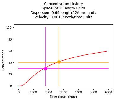
Computed concentration at time  1700  =  29.0  Target value  30.0
Computed concentration at time  2700  =  41.0  Target value  40.0

The dispersion coefficient.

The dispersion coefficient from the modeling exercise above is \(0.64~\frac{cm^2}{sec}\)

The longitudinal dispersivity.

Using equation 6.41 and a reported value for molecular diffusion of chloride in wasser of \(2.3 \times 10^{-5} ~ \frac{cm^2}{sec}\) the dispersivity is \(\alpha_l = \frac{D_l-D_d}{1 \times 10^{-3}} = \frac{0.64-2.3 \times 10^{-5}}{1 \times 10^{-3}} \)

alpha_l = (dispersion/velocity - 2.3e-5) #cm
print("Dispersivity = ",round(alpha_l,3)," centimeters")

Dispersivity =  640.0  centimeters

Comments¶

This value of dispersivity is unrealistic.

The longitudinal dispersivity using the dispersivity plot in the book

Observe that for the problem conditions we are in the lower left corner of the log-log plot where dispersivities are approximately \(\frac{1}{10} ~ to ~\frac{1}{100}\) of the path length. So for this problem \(\alpha_l = 0.5 ~to ~ 5 ~\text{centimeters}\)

The dispersion coefficient.

The dispersion coefficient is the product of dispersivity and seepage velocity (Eq. 6.7 of textbook) plus the molecular diffusion coefficient (\(D_d ~\approx~2 \times 10^{-9} \frac{cm^2}{sec}\)). For this problem

\(D_l = 0.5 \cdot 1\times~10^{-3}~\frac{cm^2}{sec} + 2 \times 10^{-9} \frac{cm^2}{sec} ~\approx~ 5.0~to~50.0 \times 10^{-4} \frac{cm^2}{sec}\)

So the dispersion coefficients in this problem are unrealistic.

Problem 2 (Problem 6-2, pg. 567)¶

Chloride (𝐶𝑙−) is injected as a continuous source into a 1-D column. The system has Darcy velocity of \(5.18 \times 10^{-3}~\frac{in}{day}\), a porosity of \(n=0.30\), and longitudinal dispersivity of \(5 m\).

Determine:

Sketch the system.
The ratio \(\frac{C}{C_0}\) at a location 0.3 meters from the injection location after 5 days of injection.
The ratio \(\frac{C}{C_0}\) at a location 0.3 meters from the injection location after 5 days of injection, if the dispersivity is 4 times larger (\(20 m\)).
Comment on the difference in results.

# Enter your solution below, or attach separate sheet(s) with your solution.

1. Sketch the system¶

Convert \(5.18 \times 10^{-3}~\frac{in}{day}\) into meters per day

\(5.18 \times 10^{-3}~\frac{in}{day} * \frac{1~ft}{12~in} * \frac{1~m}{3.28~ft} = 1.32 \times 10^{-4} \frac{m}{day}\)

Then find the pore velocity

\(u = 1.32 \times 10^{-4} \frac{m}{day} \cdot \frac{1}{0.3} = 4.4 \times 10^{-4} \frac{m}{day} \)

2. The ratio \(\frac{C}{C_0}\) at a location 0.3 meters from the injection location after 5 days of injection.¶

Apply the same modeling tool.

from math import sqrt,erf,erfc,exp  # get special math functions
#
# prototype ogatabanks function
#
def ogatabanks(c_source,space,time,dispersion,velocity):
    term1 = erfc(((space-velocity*time))/(2.0*sqrt(dispersion*time)))
    term2 = exp(velocity*space/dispersion)
    term3 = erfc(((space+velocity*time))/(2.0*sqrt(dispersion*time)))
    ogatabanks = c_source*0.5*(term1+term2*term3)
    return(ogatabanks)
#
# example inputs
#
c_source = 100.0 # source concentration
space = 3.      # how far in X-direction to extend the plot
time  = 5.       # time since release
velocity = (1.32E-04)/(0.30)    # pore velocity (in/day)
dispersion = (5)*velocity  # dispersion coefficient
#
# forward define and initialize vectors for a profile plot
#
how_many_points = 500  
deltax = space/how_many_points
x = [i*deltax for i in range(how_many_points)] # constructor notation
c = [0.0 for i in range(how_many_points)]      # constructor notation
#
# build the profile predictions
#
for i in range(0,how_many_points,1):
    c[i] = ogatabanks(c_source,x[i],time,dispersion,velocity)
#
# Import graphics routines for picture making
#
from matplotlib import pyplot as plt
#
# Build and Render the Plot
#
plt.plot(x,c, color='red', linestyle = 'solid')  # make the plot object
plt.title(" Concentration Profile \n Time: " + repr(time) + " time units \n" + " Dispersion: " + repr(dispersion) + " length^2/time units \n" + " Velocity: " + repr(velocity) + " length/time units \n") # caption the plot object
plt.xlabel(" Distance from Source ") # label x-axis
plt.ylabel(" Concentration        ") # label y-axis
#plt.savefig("ogatabanksplot.png") # optional generates just a plot for embedding into a report
plt.show() # plot to stdio -- has to be last call as it kills prior objects
plt.close('all') # needed when plt.show call not invoked, optional here
#sys.exit() # used to elegant exit for CGI-BIN use

cone = ogatabanks(c_source,0.3,time,dispersion,velocity)
print("C/Co at 0.3 meters = ",round(cone/c_source,2),)

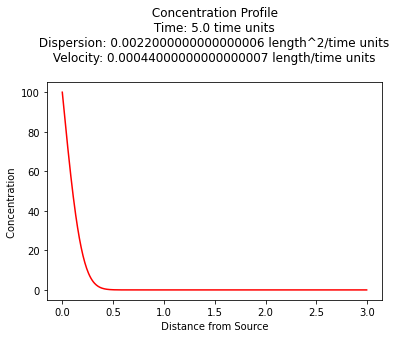
C/Co at 0.3 meters =  0.04

3. The ratio \(\frac{C}{C_0}\) at a location 0.3 meters from the injection location after 5 days of injection, if the dispersivity is 4 times larger (\(20 m\)).¶

from math import sqrt,erf,erfc,exp  # get special math functions
#
# prototype ogatabanks function
#
def ogatabanks(c_source,space,time,dispersion,velocity):
    term1 = erfc(((space-velocity*time))/(2.0*sqrt(dispersion*time)))
    term2 = exp(velocity*space/dispersion)
    term3 = erfc(((space+velocity*time))/(2.0*sqrt(dispersion*time)))
    ogatabanks = c_source*0.5*(term1+term2*term3)
    return(ogatabanks)
#
# example inputs
#
c_source = 100.0 # source concentration
space = 3.      # how far in X-direction to extend the plot
time  = 5.       # time since release
velocity = (1.32E-04)/(0.30)    # pore velocity (in/day)
dispersion = 4*(5)*velocity  # dispersion coefficient
#
# forward define and initialize vectors for a profile plot
#
how_many_points = 50  
deltax = space/how_many_points
x = [i*deltax for i in range(how_many_points)] # constructor notation
c = [0.0 for i in range(how_many_points)]      # constructor notation
#
# build the profile predictions
#
for i in range(0,how_many_points,1):
    c[i] = ogatabanks(c_source,x[i],time,dispersion,velocity)
#
# Import graphics routines for picture making
#
from matplotlib import pyplot as plt
#
# Build and Render the Plot
#
plt.plot(x,c, color='red', linestyle = 'solid')  # make the plot object
plt.title(" Concentration Profile \n Time: " + repr(time) + " time units \n" + " Dispersion: " + repr(dispersion) + " length^2/time units \n" + " Velocity: " + repr(velocity) + " length/time units \n") # caption the plot object
plt.xlabel(" Distance from Source ") # label x-axis
plt.ylabel(" Concentration        ") # label y-axis
#plt.savefig("ogatabanksplot.png") # optional generates just a plot for embedding into a report
plt.show() # plot to stdio -- has to be last call as it kills prior objects
plt.close('all') # needed when plt.show call not invoked, optional here
#sys.exit() # used to elegant exit for CGI-BIN use

cone = ogatabanks(c_source,0.3,time,dispersion,velocity)
print("C/Co at 0.3 meters = ",round(cone/c_source,2),)

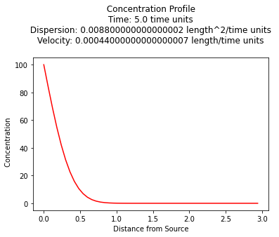
C/Co at 0.3 meters =  0.31

4. Comment on the difference in results.¶

The first condition with relatively small dispersivity exhibits about 1/7 the spread at the indicated time. The “advective” part of the transport is at location \(x_{adv} = 0.00044 \frac{m}{day} \cdot 5 \text{day} = 0.0022~meters\) hence the “front” has hardly moved.

Problem 3 (Problem 6-3, pg. 587)¶

The estimated mass from an instantaneous release of benzene is \(107 \frac{kg}{m^2}\) of a 1-D aquifer system. The aquifer has a seepage velocity of \(0.03 \frac{in}{day}\) and a longitudinal dispersion coefficient of \(9 \times 10^{-4}\frac{m^2}{day}\)

Determine:

Sketch the system.
Plot a concentration profile at \(t = 1~\text{year}\) for \(x = 0\) to \(x = 50\) inches, in 1-inch increments.
Plot a concentration history at \(x=v\times (1~\text{year})\) (this value stays constant) for \(t = 0\) to \(t = 2 \) years in \(\frac{1}{12}\)-year increments.
The maximum concentration at \(t = 1~\text{year}\) and its location.

# Enter your solution below, or attach separate sheet(s) with your solution.

1. Sketch the system.¶

Convert \(0.03 \frac{in}{day}\) into \(\frac{m}{day}\)
\(0.03 \frac{in}{day} * \frac{1~ft}{12~in} * \frac{1~m}{3.28~ft} = 0.0007622 \frac{m}{day}\)
Convert \(1 in * \frac{0.0254~m}{1~in} = 0.0254~m\)

2. Plot a concentration profile at \(t = 1~\text{year}\) for \(x = 0\) to \(x = 50\) inches, in 1-inch increments.¶

Convert \(1~in * \frac{0.0254~m}{1~in} = 0.0254~m\)

def conc(distance,time,mass,dispersion,velocity):
    import math
    term1 = math.sqrt(4.0*math.pi*dispersion*time)
    term2 = math.exp(-((distance-velocity*time)**2)/(4.0*dispersion*time))
    conc = (mass/term1)*term2
    return(conc)

thick       = 1.0
width       = 1.0
length      = 1.0
c0          = 107.0 # kg/m^3
volume      = thick*width*length
porosity    = 1.0
mass        = (c0*volume)/(porosity)
dispersion  = 9e-04 #m^2/day
velocity    = 0.0007622 #m/day
deltax      = 0.0254 #inches as meters
x = [] #inches as meters
for i in range(50):
    x.append(float(i)*deltax)
time        = 365.0 #years as days
c = [0 for i in range(50)] #concentration 
for i in range(50):
    c[i]=conc(x[i],time,mass,dispersion,velocity)
#
# Import graphics routines for picture making
#
from matplotlib import pyplot as plt
#
# Build and Render the Plot
#
plt.plot(x,c, color='red', linestyle = 'solid')  # make the plot object
plt.title(" Concentration Profile \n Time: " + repr(time) + " time units \n" + " Dispersion: " + repr(dispersion) + " length^2/time units \n" + " Velocity: " + repr(velocity) + " length/time units \n") # caption the plot object
plt.xlabel(" Distance from Source ") # label x-axis
plt.ylabel(" Concentration        ") # label y-axis
#plt.savefig("ogatabanksplot.png") # optional generates just a plot for embedding into a report
plt.show() # plot to stdio -- has to be last call as it kills prior objects
plt.close('all') # needed when plt.show call not invoked, optional here
#sys.exit() # used to elegant exit for CGI-BIN use
print("Center of Distribution Position : ",round(time*velocity,2)," length units")

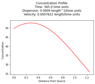
Center of Distribution Position :  0.28  length units

3. Plot a concentration history at \(x=v\times (1~\text{year})\) (this value stays constant) for \(t = 0\) to \(t = 2 \) years in \(\frac{1}{12}\)-year increments.¶

def conc(distance,time,mass,dispersion,velocity):
    import math
    term1 = math.sqrt(4.0*math.pi*dispersion*time)
    term2 = math.exp(-((distance-velocity*time)**2)/(4.0*dispersion*time))
    conc = (mass/term1)*term2
    return(conc)

thick       = 1.0
width       = 1.0
length      = 1.0
c0          = 107.0 # kg/m^3
volume      = thick*width*length
porosity    = 1.0
mass        = (c0*volume)/(porosity)
dispersion  = 9e-04 #m^2/day
velocity    = 0.0007622 #m/day
deltat      = (1/12)*365 #
howmany = 2*365/deltat 
howmany = int(howmany)
#print(howmany)

t = [] #days
for i in range(howmany*2):
    t.append(float(i)*deltat)
    if t[i] == 0: # trap zero time to prevent divide by zero
        t[i]= 0.00000001
    
distance        = 365.0*velocity #years as days

c = [0 for i in range(howmany*2)] #concentration 

for i in range(howmany*2):
    c[i]=conc(distance,t[i],mass,dispersion,velocity)
#
# Import graphics routines for picture making
#
from matplotlib import pyplot as plt
#
# Build and Render the Plot
#
plt.plot(t,c, color='red', linestyle = 'solid')  # make the plot object
plt.title(" Concentration History \n Distance: " + repr(distance) + " length units \n" + " Dispersion: " + repr(dispersion) + " length^2/time units \n" + " Velocity: " + repr(velocity) + " length/time units \n") # caption the plot object
plt.xlabel(" Elapsed Time (days) ") # label x-axis
plt.ylabel(" Concentration        ") # label y-axis
plt.plot([365,365],[0,c0])
plt.plot([365*2,365*2],[0,c0])
plt.text(365,100,"  year 1")
plt.text(365*2,100,"  year 2")
#plt.savefig("ogatabanksplot.png") # optional generates just a plot for embedding into a report
plt.show() # plot to stdio -- has to be last call as it kills prior objects
plt.close('all') # needed when plt.show call not invoked, optional here
#sys.exit() # used to elegant exit for CGI-BIN use
print("Center of Distribution Position : ",round(time*velocity,2)," length units")

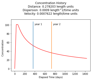
Center of Distribution Position :  0.28  length units

4. The maximum concentration at \(t = 1~\text{year}\) and its location.¶

def conc(distance,time,mass,dispersion,velocity):
    import math
    term1 = math.sqrt(4.0*math.pi*dispersion*time)
    term2 = math.exp(-((distance-velocity*time)**2)/(4.0*dispersion*time))
    conc = (mass/term1)*term2
    return(conc)

thick       = 1.0
width       = 1.0
length      = 1.0
c0          = 107.0 # kg/m^3
volume      = thick*width*length
porosity    = 1.0
mass        = (c0*volume)/(porosity)
dispersion  = 9e-04 #m^2/day
velocity    = 0.0007622 #m/day
deltax      = 0.0254 #inches as meters
x = [] #inches as meters
for i in range(365):
    x.append(float(i)*deltax)
time        = 365.0 #years as days
c = [0 for i in range(365)] #concentration 
for i in range(365):
    c[i]=conc(x[i],time,mass,dispersion,velocity)
    
#for i in range(365):
#    print(round(x[i],3),round(c[i],3))

    
xmax = velocity*time
cmax = conc(xmax,time,mass,dispersion,velocity)

print(" Maximum at time : ",round(time,3) ," days\n     at location : ", round(xmax/deltax,3)," inches\n      is :" ,round(cmax,3)," ppm ")

 Maximum at time :  365.0  days
     at location :  10.953  inches
      is : 52.664  ppm 

F23 Exercise Set 2

F23 Exercise Set 3

Groundwater Transport Phenomena

F23 ES2 Solution Sketch¶

Purpose :¶

Assessment Criteria :¶

Problem 1 (Problem 6-1, pg. 567)¶

Enter your solution below, or attach separate sheet(s) with your solution.¶

Comments¶

Problem 2 (Problem 6-2, pg. 567)¶

1. Sketch the system¶

2. The ratio \(\frac{C}{C_0}\) at a location 0.3 meters from the injection location after 5 days of injection.¶

3. The ratio \(\frac{C}{C_0}\) at a location 0.3 meters from the injection location after 5 days of injection, if the dispersivity is 4 times larger (\(20 m\)).¶

4. Comment on the difference in results.¶

Problem 3 (Problem 6-3, pg. 587)¶

1. Sketch the system.¶

2. Plot a concentration profile at \(t = 1~\text{year}\) for \(x = 0\) to \(x = 50\) inches, in 1-inch increments.¶

3. Plot a concentration history at \(x=v\times (1~\text{year})\) (this value stays constant) for \(t = 0\) to \(t = 2 \) years in \(\frac{1}{12}\)-year increments.¶

4. The maximum concentration at \(t = 1~\text{year}\) and its location.¶