1. Introduction

Course Website

http://54.243.252.9/ce-5319-webroot/

Machine learning is a branch of artificial intelligence (AI) that enables computers to learn patterns and make decisions without being explicitly programmed. Instead of following predefined rules, machine learning models analyze data, recognize trends, and improve their performance over time. This ability to “learn from experience” is what makes machine learning a powerful tool across various industries, including civil engineering, where it can assist in predictive modeling, structural analysis, flood forecasting, and more.

Think of machine learning as the missing link between traditional computing and true artificial intelligence. If you’ve seen movies like Ex Machina, Transcendence, or I, Robot, you’ve already encountered fictional depictions of AI evolving beyond predefined tasks. While we’re not quite at the level of sentient machines, modern applications of machine learning—such as self-driving cars, facial recognition, and predictive maintenance in infrastructure—demonstrate how far we’ve come.

In this course, we’ll focus on practical, example-driven applications of machine learning tailored for civil engineers. You’ll learn how to:

• Prepare and analyze real-world engineering datasets, such as sensor readings, environmental data, and structural performance metrics.

• Build machine learning models that can classify, predict, and optimize engineering solutions.

• Use Python-based tools and frameworks like scikit-learn, pandas, and tensorflow to implement data-driven approaches.

By the end of this course, you should have a rudimentary understanding of theory and practice behind machine learning, and you’ll be able to apply it to real-world civil engineering challenges and automate complex decision-making processes.

Note

The chapter/lesson layout is intentional — Readings and references are not an afterthought, but are an integral part of the lesson; so I choose to lead with them! Videos are next, then my content. It’s an odd structure when compared to convetional textbooks, but given its an online book anyway, I have artistic freedom to do so. The required and recomended books are inexpensive, so really no excuse (except laziness) to get copies.

Readings/References

1. Burkov, A. (2019) The One Hundred Page Machine Learning Book Required Textbook (All references to pages are from the purchased version of the book; you may have to search the “free” version to find the referenced topic)

2. Rashid, Tariq. (2016) Make Your Own Neural Network. Kindle Edition. Required Textbook

3. Chan, Jamie. Machine Learning With Python For Beginners: A Step-By-Step Guide with Hands-On Projects (Learn Coding Fast with Hands-On Project Book 7) (p. 5-7). Kindle Edition. Recomended Book

4. Uddameri, V. (2019) Overview and Objectives. Lecture Notes for CE 5319 Fall 2021

5. Uddameri, V. (2019) Installing Anaconda and RStudio. Lecture Notes for CE 5319 Fall 2021

6. Shai Shalev-Shwartz (2014) Selected Lecture Notes from “Understanding Machine Learning” at Hebrew University of Jerusalem

7. Thevapalan, Arunn (2021). The Machine Learning Workflow Explained (and How You Can Practice It Now). Towards Data Science Blog

8. Computational and Inferential Thinking Ani Adhikari and John DeNero, Computational and Inferential Thinking, The Foundations of Data Science, Creative Commons Attribution-NonCommercial-NoDerivatives 4.0 International (CC BY-NC-ND) Chapter 1

9. Learn Python the Hard Way (Online Book) Recommended for beginners who want a complete course in programming with Python.

10. LearnPython.org (Interactive Tutorial) Short, interactive tutorial for those who just need a quick way to pick up Python syntax.

11. How to Think Like a Computer Scientist (Interactive Book) Interactive “CS 101” course taught in Python that really focuses on the art of problem solving.

12. How to Learn Python for Data Science, The Self-Starter Way

13. OpenAI. (2025). Introduction to machine learning. Interactive session to assist with contents in Machine Learning by Example for Civil Engineers. Retrieved from ChatGPT.

Videos

Why study machine learning?

The availability of big data is transforming all professions, including Civil, Environmental, and Construction Engineering. Data-driven tools and algorithms have the promise to model nonlinear civil engineering phenomena and extract information that is not possible through traditional modeling methods.

Machine learning is a fast growing field and its use in civil engineering will likely become routine in the next few years. The primary objective of this course is to provide a practical introduction and exposure to selected ML applications in Civil Engineering.

Note

The title of this JupyterBook is “Machine Learning by Example for Civil Engineers.” The intent is to indroduce various concepts, then show an example. The two required textbooks are listed above; they go more into underlying theory of the various methods employed.

Learning Methods

A brief tangent about learning methods in Biological Inference Engines (us humans) versus Mechanical Inference Engines (computers and their AI programs).

Feynman Learning Technique

The Feynman Technique is a learning strategy named after the famous physicist Richard Feynman, who was known for his ability to explain complex concepts in simple, easy-to-understand terms. This technique emphasizes understanding through simplification and self-explanation. It consists of four key steps designed to help you deeply understand a topic and identify any gaps in your knowledge. Here’s how it works:

1. Choose a Concept: Start by selecting the topic or concept you want to learn. It could be anything from a scientific principle to a technical skill or a theory. The idea is to focus on something specific that you wish to master.

2. Teach it to the President (aka Child): Pretend you’re teaching the concept to someone who has no background knowledge, such as a child. The goal is to break the concept down into the simplest possible terms. Avoid jargon or overly technical language. By doing this, you force yourself to clarify your understanding. If you can explain a complex idea in simple language, it’s a sign you truly understand it.

3. Identify Gaps and Go Back to the Source: As you attempt to explain the concept, you may discover areas where your explanation feels incomplete or confusing. These are the gaps in your understanding. When you find them, return to the source material—books, notes, or any reference—and review the sections you don’t fully grasp. The key is to refine your understanding by identifying and filling these gaps.

4. Simplify and Use Analogies: Once you’ve filled the gaps, simplify your explanation again, but this time refine it by making it even clearer. Use analogies and comparisons to make the concept easier to understand. Analogies are powerful tools that help relate complex ideas to familiar concepts, making them more accessible.

Why the Feynman Technique seems to Work:

• Active Learning: This technique encourages active engagement with the material rather than passive consumption. You are not just reading or listening—you are breaking down, teaching, and critically analyzing the concept.

• Understanding vs. Memorization: The Feynman Technique forces you to truly understand a concept rather than memorize it. If you can’t explain it simply, it shows you haven’t fully grasped it yet.

• Identification of Weaknesses: By trying to explain the topic in simple terms, you quickly uncover any parts of the material that you don’t understand well.

• Effective Communication: The technique not only helps you learn but also improves your ability to communicate ideas clearly to others, a skill valuable in teaching, leadership, and many professional fields.

Example:

Suppose you’re trying to learn Newton’s First Law of Motion. Using the Feynman Technique, you would start by writing out the law in your own words as if explaining it to a child: “Objects keep moving or stay still unless something pushes or pulls them.” If you struggle with this simplification, you would go back to the material to clarify your understanding, then return and explain it more clearly.

The Feynman Technique is a practical, powerful method for mastering difficult subjects and can be applied to almost any area of study.

Note

When I was a drill sergeant in the U.S. Army, we used a doctrine at the time called “Method of Learning Concept”, which is essentially the same thing - outcomes were easier to define (Mission Accomplishmet and Retention of Assets (aka not becoming unalive in the process of mission accomplishment).

U.S. Army’s Method of Learning Concept Overview

The U.S. Army’s Method of Learning Concept (also called Crawl-Walk-Run method) was designed to train soldiers for the practical application of skills and knowledge in real-world scenarios. The focus is on incremental learning through experience and repetition, combined with immediate feedback. It is a structured approach often used in the military and emphasizes action-based learning in phases:

• Crawl Phase (Basic Learning): Introduce the material, concept, or skill in a simplified form. Soldiers receive theoretical knowledge, often through briefings, instruction, or reading materials. Learning is foundational, focused on understanding the basics before moving on to more complex elements.

• Walk Phase (Hands-On Practice): Transition to practical application and drills. Soldiers practice skills or apply knowledge under controlled conditions. Mistakes are expected, and learning happens through hands-on experience with increasing difficulty. Instructors provide feedback and correct errors as they happen.

• Run Phase (Full Application): Apply the learned skills or knowledge in real-time, high-pressure environments (simulated combat or field exercises). Soldiers must demonstrate competence and adaptability. The goal is to prepare them for real-world scenarios where the learned concepts will be applied under stress.

Comparison

Aspect	Feynman Technique	U.S. Army’s Method of Learning Concept
Focus	Conceptual clarity by simplifying and teaching complex ideas in a way that anyone can understand.	Practical skills and readiness, learning through phased progression and real-world application.
Learning Style	Self-directed, with an emphasis on self-explanation and refining understanding by teaching others or oneself.	Instructor-led, action-based with structured phases: basic learning, practical application, and real-world simulation.
Application	Best suited for mastering intellectual, academic, or technical knowledge by focusing on why and how something works.	Designed for learning skills and procedures in a stepwise fashion, with increasing complexity, leading to readiness for real-world execution (e.g., military or high-stakes environments).
Feedback Mechanism	Feedback occurs when learners identify gaps in their own understanding during the teaching process.	Immediate, instructor-provided feedback during hands-on practice. Mistakes are corrected as they occur.
Learning Pace	Flexible, with learners progressing at their own pace by revisiting material as needed.	Structured, with clear progression through phases (crawl-walk-run), often tied to a timeline or mission readiness.
Learning Outcome	Learners can explain concepts clearly and simply, which signifies true mastery of the topic.	Learners can apply skills effectively in stressful or practical situations, often preparing for real-world action.
Key Strength	Identifying gaps in knowledge through the act of teaching, leading to deep understanding.	Building practical competence by transitioning from theory to real-world application under pressure.

Which is Better for Learning?

• The Feynman Technique is particularly useful for academic and intellectual fields where deep understanding and explanation of complex ideas are necessary. It’s excellent for self-learners or people studying theoretical or technical subjects.

• The Army’s Method is designed for learning practical, hands-on skills in high-stakes environments. It ensures that the learner can execute tasks effectively in real-world conditions, which is critical for fields requiring physical performance, such as military, engineering operations, or emergency response.

Summary

The Feynman Technique is considered more suited for learning abstract or conceptual material, where explaining and teaching lead to deeper understanding. In contrast, the U.S. Army’s Method emphasizes skill acquisition and real-world application through incremental practice, feedback, and full-speed execution. Both methods are powerful, but their effectiveness depends on the type of learning goal—whether you’re trying to understand a concept intellectually or master a skill through action.

Human vs. Machine Learning: A Comparative Perspective

Humans and machines both aim to learn from data or experiences, but their mechanisms and approaches are fundamentally different:

1. Biological Inference (Human Learning)

   Structure: Human learning relies on a complex network of neurons in the brain. Information is processed hierarchically, building upon previous knowledge. Learning Process: Humans learn actively and contextually, leveraging intuition, emotions, and creativity. Key aspects include: Experiential Learning: Gaining knowledge through direct experiences. Analogical Reasoning: Drawing comparisons between known and unknown concepts. Adaptive Understanding: Quickly adjusting to new or unforeseen situations.

2. Mechanical Inference (Machine Learning)

   Structure: Machine learning models are based on mathematical algorithms and artificial neural networks, mimicking some aspects of human neural processing but on a vastly different scale. Learning Process: Machines learn systematically and repetitively: Data-Driven: Machines need large datasets to generalize and infer patterns. Optimization Algorithms: Models minimize error through iterative adjustments, such as gradient descent. Feature Engineering: Machines rely on humans to identify and preprocess relevant data characteristics for improved learning. Generalization: The ability to apply learned patterns to unseen data depends on avoiding overfitting during training.

Key Comparisons

Aspect	Human Learning	Machine Learning
Knowledge Basis	Builds on innate understanding and prior knowledge.	Starts from scratch; requires explicit data.
Flexibility	Highly adaptable; handles new situations intuitively.	Limited to learned patterns; struggles with outliers.
Efficiency	Can infer meaning from limited data points.	Needs vast quantities of data for accuracy.
Errors	Prone to bias and emotional distractions.	Prone to bias from data quality or algorithmic limitations.
Feedback	Can self-correct through reflection or external feedback.	Learns through defined loss functions and adjustments.

Synergies Between Human and Machine Learning

While humans excel in conceptual thinking, machines thrive in processing and analyzing large datasets quickly. Together, these strengths can be leveraged for tasks such as:

• Augmented Decision-Making: Humans define objectives; machines analyze data.

• Creative Problem Solving: Machines generate novel solutions based on patterns, which humans refine.

• Automation of Repetitive Tasks: Machines handle routine operations, freeing humans for creative and strategic efforts.

By understanding these distinctions and synergies, engineers can effectively harness the power of machine learning to complement human expertise in solving complex problems.

Learning Types

Machine learning can be broadly categorized into three major approaches: Supervised Learning, Unsupervised Learning, and Semi-Supervised Learning. Each approach differs in how data is presented to the learning algorithm and the role of labeled information.

---

Supervised Learning

Supervised learning involves training an algorithm using a dataset where both the inputs and their desired outputs (labels) are provided. The goal is for the algorithm to learn a mapping function that correctly associates inputs with outputs.

A common example is image classification — such as distinguishing between images of cats and dogs. The algorithm is trained with thousands of labeled images, where each image is paired with a category label (“dog” or “cat”). Over time, the model learns to recognize features that define each category, enabling it to classify new, unseen images with high accuracy.

Civil Engineering Examples

1. Pavement Condition Assessment: In pavement condition monitoring, supervised learning is used to classify road surfaces based on images or sensor data. Engineers provide labeled examples of “Good,” “Moderate,” and “Poor” pavement conditions. The trained model can then automatically classify roads, helping prioritize maintenance and repairs.

2. Water Quality Prediction: Supervised learning can predict water contamination levels based on sensor data (e.g., pH, turbidity, dissolved oxygen). Historical data with known contamination levels is used to train the model, which can then estimate water quality in unmonitored locations.

---

Unsupervised Learning

In unsupervised learning, the algorithm is provided only with inputs, without any explicit labels or desired outputs. Instead of learning to classify, the algorithm must find patterns, relationships, or structures within the data on its own.

Using the same cat-and-dog example, an unsupervised learning algorithm would be given thousands of images without labels. The model would then attempt to identify similarities and groupings based on features like shape, size, or fur texture — effectively clustering the images into distinct categories without being explicitly told what a cat or a dog is.

Unsupervised learning is widely used in:

• Anomaly detection (e.g., identifying structural defects in engineering systems)

• Customer segmentation (e.g., grouping users by behavior for targeted marketing)

• Dimensionality reduction (e.g., simplifying large datasets for visualization)

Civil Engineering Examples

1. Bridge Defect Clustering: Unsupervised learning can analyze sensor readings from bridges to detect unusual vibration patterns. The algorithm clusters different bridge sections based on their response to traffic loads, highlighting areas that may require further structural assessment.

2. Air Pollution Pattern Detection: An unsupervised algorithm can process air quality sensor data from multiple locations, grouping sites based on pollution patterns. This helps identify regional air pollution trends, such as industrial zones contributing to high particulate matter levels.

---

Semi-Supervised Learning (SSL)

Semi-supervised learning (SSL) is a hybrid approach that combines aspects of both supervised and unsupervised learning. The algorithm is trained on a small set of labeled data alongside a much larger set of unlabeled data.

For example, consider web page classification — categorizing websites into topics such as “shopping” or “news.” Labeling every website manually would be impractical and expensive. Instead, an SSL model can be trained using a small, manually labeled subset of websites, then generalize its learning across thousands of unlabeled websites by identifying similarities.

SSL is particularly useful when:

• Labeled data is expensive or difficult to obtain (e.g., medical imaging, where expert labeling is costly).

• Large amounts of unlabeled data exist, and partial supervision can improve accuracy.

Civil Engineering Example(s)

1. Traffic Flow Classification: Semi-supervised learning can classify traffic congestion levels using a combination of labeled and unlabeled traffic camera footage. A small portion of the images are labeled as “High Traffic” or “Low Traffic,” and the model generalizes patterns across thousands of unlabeled images.

2. Floodplain Mapping: Floodplain maps require extensive manual labeling of flood-prone zones. SSL can use a few labeled flood records alongside unlabeled hydrological data to improve flood risk predictions.

---

Reinforcement Learning (RL)

Reinforcement Learning (RL) is distinct from Supervised, Unsupervised, and Semi-Supervised Learning, but it could be considered a fourth category in the taxonomy. Unlike the other types, RL focuses on decision-making rather than direct pattern recognition.

Where Does Reinforcement Learning Fit?

• Different from Supervised Learning → In supervised learning, models learn from fixed labeled data. In contrast, RL learns by interacting with an environment and receiving rewards or penalties.

• Different from Unsupervised Learning → RL does not simply find structure in data. Instead, it actively explores an environment to maximize a reward.

• Different from Semi-Supervised Learning → SSL relies on a small set of labeled data, while RL relies purely on feedback (rewards) from the environment.

Thus, Reinforcement Learning is its own category and does not fit neatly into the previous three. It could be added as a separate section:

Reinforcement Learning (RL)

Reinforcement learning is a machine learning approach where an agent learns by interacting with an environment and receiving feedback in the form of rewards or penalties. The goal is to maximize cumulative rewards over time.

Unlike supervised learning, where models learn from labeled examples, RL learns through trial and error. This makes it well-suited for problems involving sequential decision-making, where an agent must decide the best action at each step.

Civil Engineering Example(s)

1. Traffic Signal Optimization: Reinforcement learning can be used to optimize traffic signals at intersections. The RL agent continuously adjusts signal timing based on traffic conditions, minimizing congestion and wait times.

2. Smart Irrigation Systems: In water resource management, RL can be applied to optimize irrigation schedules. The RL agent decides when and how much to irrigate based on weather conditions, soil moisture levels, and water availability, reducing waste and improving efficiency.

Comparison of Learning Types

Learning Type	Labeled Data?	Representative Use Cases
Supervised Learning	Yes	Pavement assessment, water quality prediction
Unsupervised Learning	No	Bridge defect clustering, air pollution patterns
Semi-Supervised Learning	Mixed	Traffic flow classification, floodplain mapping
Reinforcement Learning	No (Reward-based)	Traffic signal optimization, smart irrigation

Note

Reinforcement Learning and Environmental Feedback

Reinforcement Learning (RL) inherently involves feedback from the environment, distinguishing it from other learning types.

How RL Uses Environmental Feedback

• Feedback Loop → RL operates in a continuous sense-decide-act loop, where an agent interacts with the environment, observes the results of its actions (senses the state), and adjusts its behavior to maximize cumulative rewards.

• Sensors as Inputs** → In practical applications, environmental sensors provide the state of the system, guiding decision-making.

• Reward Signals → The agent receives reward signals based on performance. For example:

  • A traffic control RL system receives a reward for reducing congestion.

  • A smart irrigation RL system receives a reward for minimizing water use while maintaining soil moisture.

Contrast with Supervised Learning

Aspect	Supervised Learning	Reinforcement Learning
Learning Data	Fixed labeled dataset	Learns dynamically from feedback
Environment Role	No interaction with environment	Actively interacts with environment
Error Feedback	Direct from dataset labels	Indirect via rewards & penalties
Example	Image classification	Robot navigating terrain

Civil Engineering Example(s)

1. Adaptive Structural Control

• Sensors detect wind forces or seismic activity on a bridge.

• The RL agent adjusts dampers or counterweights based on feedback to minimize vibrations.

2. Autonomous Floodgate Management

• Water level sensors detect rising river levels.

• The RL agent adjusts floodgate openings to balance flood prevention and reservoir storage.

---

Illustration: Reinforcement Learning Feedback Loop

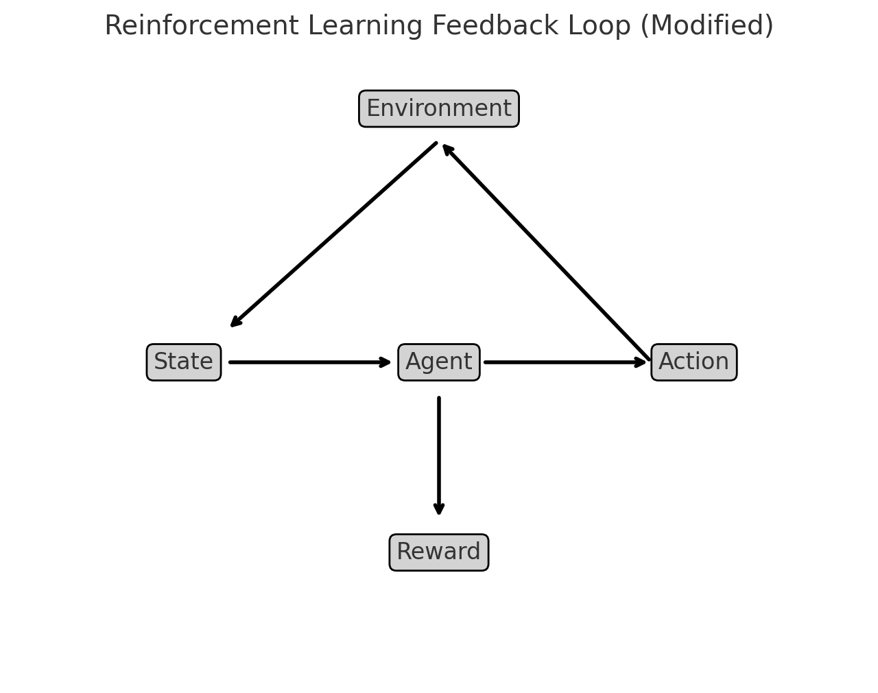
OpenAI. (2025). Reinforcement learning feedback loop [Diagram]. Generated using Matplotlib.

How to Interpret the Diagram:

• The Agent interacts with the Environment by taking an Action.

• The Environment responds by providing a State (new conditions) and a Reward (feedback on how good or bad the action was).

• The Agent learns from this cycle, refining its actions over time to maximize cumulative rewards.

The reward is a bidirectional operation. The agent gets its reward based on state and action costs and in the next decision adjusts the action to improve the reward. This type of feedback loop makes RL well-suited for dynamic control systems like adaptive structural control or autonomous flood management.

Is machine learning just a clever rebranding of older concepts and technologies of statistical data modeling, with some new tools (ANN, SVM …) included?

The question touches on a debate that has persisted in academic and professional circles. Machine learning (ML) indeed shares deep roots with statistical modeling, and to some extent, it can be seen as an evolution of traditional methods rather than an entirely new field. Here’s a nuanced perspective:

1. Shared Roots and Rebranding

   • Statistical Foundations: Many machine learning methods are grounded in classical statistics. For example: Linear regression is a precursor to algorithms like logistic regression, a staple in both statistics and ML. Probabilistic models (e.g., Bayesian inference) are directly used in ML under the guise of tools like Naive Bayes classifiers.

   • Terminology Shift: In many cases, what statisticians called “predictive modeling” is now referred to as supervised learning. This rebranding aligns with the computational and engineering focus of ML rather than the theoretical focus of statistics.

2. What Makes ML Different? While ML builds on statistical principles, it diverges in scope and emphasis in the following ways:

   • Scalability and Automation: Traditional statistical models are often limited to specific hypotheses tested on relatively small datasets. Machine learning focuses on scalability, with algorithms designed to process massive datasets autonomously.

   • Nonlinear Models: Tools like Artificial Neural Networks (ANNs), Support Vector Machines (SVMs), and ensemble methods (e.g., Random Forests) go beyond the linear assumptions of many traditional statistical models, making them suitable for highly complex patterns.

   • Performance Orientation: In statistics, understanding the model and its assumptions is paramount. In ML, the focus is often on predictive accuracy, sometimes at the expense of interpretability.

   • Automation of Feature Learning: Modern ML techniques, such as deep learning, can automatically extract relevant features from raw data (e.g., convolutional layers in neural networks for image recognition), reducing the need for manual feature engineering.

3. New Tools vs. Old Concepts

   • Innovative Techniques: Some ML tools represent genuine innovation: Reinforcement learning extends beyond traditional data modeling, focusing on decision-making in dynamic environments. Transfer learning and unsupervised learning have relatively less emphasis in classical statistics.

   • Computational Advances: The practical application of ML owes much to advancements in computational power (e.g., GPUs) and the availability of big data, which were not as accessible during the formative years of statistical data modeling.

4. Complementary or Redundant?

   • Overlap Exists: For many applications, the distinction between ML and traditional statistics is blurred. For instance, linear regression is a tool in both fields.

   • Complementary Strengths: Machine learning excels in predictive tasks where the relationships in data are complex and nonlinear, while statistics shines in inference, where the goal is understanding causality and uncertainty.

5. Is It Just Clever Rebranding? It depends on the perspective:

   • Yes, in some contexts: Many ML techniques can be seen as extensions or computational implementations of statistical ideas, repackaged with new terminology for a broader audience (e.g., engineers, computer scientists).

   • No, for others: The emphasis on automation, scalability, and performance, coupled with novel approaches like deep learning, represents a significant departure from traditional statistical methods.

Note

Machine learning is not just a rebranding of older concepts—it is better understood as a natural progression that integrates statistical theory, computational advancements, and the demands of the data-rich modern world. While it shares much with traditional statistical modeling, ML expands the toolbox, enabling practitioners to tackle problems that were previously infeasible due to computational or data limitations.

Computational Environment

The course itself is mathematically oriented and will require developing scripts (computer programs). The default computational environment is a Jupyter Notebook running an iPython kernel.

Note

In fact this on-line document is a collection of Jupyter Notebooks rendered using a program called Sphinx that converts the notebooks into a website (which you are now accessing). For me the author its cool because I just make notebooks and bind them at my leisure (there are some nuances to get figures into the books and embedding code - but its not too hard to do so. Jupyter as a literate programming environment is quite useful even outside of the University.

Jupyter Notebooks

To follow along with the examples in these notes, you need to have access to Jupyter Notebook. Jupyter Notebook is an open-source interactive computational environment that is based on a server-client structure. It includes a web server and a web application that works like an integrated development environment (IDE). This web application allows us to create Jupyter Notebook documents (commonly referred to simply as notebooks or IPYNB files) that consist of code, text, and images. To use Jupyter notebook, we have several options:

1. Anaconda

The first option is to install an instance on your own system. The easiest way to do that is to install a software distribution known as Anaconda. Anaconda comes with over 250 packages pre-installed, including NumPy, pandas, Matplotlib, and Scikit-Learn, all of which we’ll be using in this book. In addition, it includes many useful applications and IDEs,such as the Jupyter Notebook application mentioned above. This is probably the easiest approach if you already have a laptop and want to work offline.

2. Google Colaboratory

The second option to access Jupyter Notebook is to use Google Colab (short for Google Colaboratory). Google Colab is a free cloud-based Jupyter Notebook environment hosted by Google that requires no installation and offers free access to online computing resources. However, you need to be connected to the internet when you use Google Colab. This connection is mainly used to run the code and does not consume much data.

Note

Most of the scripts in this book can be cut-and-pasted into a Colab instance and seem to run as expected. The only realistic limitation is likely bandwidth (and possibly storage for big-data). Otherwise this is a good compromise and training environment for this course. Files need to be uploaded each connection and are destroyed when you disconnect, so you may need to write code to get files every time. Anyway it is a useable option.

3. Build from Repositories

A third option is to build a JupyterLab Server on a machine you own (such as AWS Virtual Private Server; Raspberry Pi runing on a home network, or similar set-up) and essentially replicate a Colab-type environment. This option is not for the faint of heart; it it the structure I used for this document. If your host machine is running Linux a good starting place is Installing Jupyter. This method is most definitely not point-and-click but can build a fully capable system on hardware you can control and scale.

Note

The hardware requirements are modest. This JupyterBook is developed on my home machine which is a Raspberry Pi 4B 8GB SBC using a 256GB MicroSD card to house the OS and data files. At current prices the hardware cost is about $240 so hardware is not a limiting issue.

Here’s a price list for your own JupyterHub server

Item	Price
Raspberry Pi 4B 8GB	$184.99
Power Supply	$10.99
Micro SD Card Class 10 or faster	$34.99
Total	$230.97

If you can find the Raspberry Pi at the MSRP ($75) you will fare even better.

Build Notes for Raspberry Pi running Ubuntu

Here are the build commands to make your own JupyterHub on a raspberry pi

First you will want a web server, might as well install R to see if we can get it into kernel list

# install and configure apache
sudo apt install apache2
sudo systemctl status apache2
sudo systemctl stop apache2
# install R
sudo apt-get install r-base-core
sudo apt-get install r-base

Next some Jupyter specific instructions

# install and configure JupyterHub
sudo apt install -y python3-pip
sudo apt install -y build-essential libssl-dev libffi-dev python3-dev
sudo apt-get install python3-venv
sudo python3 -m venv /opt/jupyterhub/
sudo apt install nodejs npm
sudo npm install -g configurable-http-proxy
sudo /opt/jupyterhub/bin/python3 -m pip install wheel
sudo /opt/jupyterhub/bin/python3 -m pip install jupyterhub jupyterlab
sudo /opt/jupyterhub/bin/python3 -m pip install ipywidgets
sudo mkdir -p /opt/jupyterhub/etc/jupyterhub/
cd /opt/jupyterhub/etc/jupyterhub/
sudo /opt/jupyterhub/bin/jupyterhub --generate-config
EDIT THE CONFIG "c.Spawner.default_url = '/lab'"
sudo mkdir -p /opt/jupyterhub/etc/systemd
sudo nano /opt/jupyterhub/etc/systemd/jupyterhub.service
INSERT <--
[Unit]
Description=JupyterHub
After=syslog.target network.target

[Service]
User=root
Environment="PATH=/bin:/usr/local/sbin:/usr/local/bin:/usr/sbin:/usr/bin:/opt/jupyterhub/bin"
ExecStart=/opt/jupyterhub/bin/jupyterhub -f /opt/jupyterhub/etc/jupyterhub/jupyterhub_config.py

[Install]
WantedBy=multi-user.target
-->
sudo ln -s /opt/jupyterhub/etc/systemd/jupyterhub.service /etc/systemd/system/jupyterhub.service
sudo systemctl daemon-reload
sudo systemctl enable jupyterhub.service
sudo systemctl status jupyterhub.service
sudo systemctl start jupyterhub.service

If you want the mathematical typesetting to work, you also need a Latex engine.

If you want to be able to build PDF renderings of notebooks a few added dependencies need to be added:

--> dependencies to get nbconvert to work (this is a list, build a few at a time until it works)---------
  texlive-lang-french texlive-latex-base texlive-latex-recommended
  python-pil-doc python3-pil-dbg python-pygments-doc ttf-bitstream-vera
  python-pyparsing-doc dvipng imagemagick-6.q16 latexmk libjs-mathjax
  python3-sphinx-rtd-theme python3-stemmer sphinx-doc texlive-fonts-recommended
  texlive-latex-extra texlive-plain-generic sgml-base-doc debhelper
  gdb-doc python3-doc python3-pil.imagetk python3-gdbm-dbg python3-tk-dbg
  ghostscript-x imagemagick-doc autotrace cups-bsd | lpr | lprng enscript ffmpeg gimp 
  gnuplot grads graphviz hp2xx html2ps
  libwmf-bin mplayer povray radiance sane-utils transfig ufraw-batch colord libfftw3-bin 
  libfftw3-dev libgd-tools gvfs fonts-mathjax-extras fonts-stix libjs-mathjax-doc inkscape 
  libjxr-tools librsvg2-bin libwmf0.2-7-gtk www-browser zathura-ps zathura-djvu zathura-cb
<---- end dependencies ----

Build a desktop

# install Xfce and TightVNC for a desktop
sudo apt update
sudo apt install xfce4 xfce4-goodies
sudo apt install tightvncserver

Into ~/.vnc/xstartup 

---add--->

#!/bin/bash
xrdb \$HOME/.Xresources
startxfce4 &

Next open holes in the firewall for everything to work

sudo ufw allow from 192.168.1.1/24 to any port 5901 
sudo ufw allow 'Apache Full'
sudo ufw allow 'OpenSSH'

At this point you would be about 3-5 hours into the build, and should have a useable JupyterHub (a lot like the Colaboratory, but you own it - warts and all!

Why Python?

A skilled user can install an R kernel into Jupyter and run R scripts, or just run R directly. I tend to use python because I also teach undergraduate programming in python and don’t want to confuse myself. I am literate in R, but prefer python slightly. So we will default to python unless something is way easier in R (and will probably still do a mixed language call in that instance!).

While no prior experience with Python or R are required, familiarity with programming concepts as covered in ENGR 1330: Computational Thinking with Data Science and statistical concepts in CE 5315: Probabilistic Methods for Engineers is useful, as are the concepts and applications in CE 5310 Numerical Methods in Engineering.

The two computational environments can be downloaded and installed from

Software Title	Internet Source Link
Anaconda: A modeling environment that integrates Jupyter and Python	https://www.anaconda.com/
R statistical and programming environment	https://cran.r-project.org/

What is Machine Learning?

Machine learning is a terminology for computer programs that provide computers the ability to perform a task without being explicitly programmed for that task.

As an example, suppose we want to sort emails into promotional and non-promotional emails. In conventional programming, we can do this using a set of hard-coded rules or conditional statements. For instance, one possible rule is to classify an email as promotional if it contains the words “Discount”, “Sale”, or “Free Gift”. We can also classify an email as non-promotional if the email address includes “.gov” or “.edu”. The problem with such an approach is that it is challenging to come up with the rules.

For instance, while most emails from addresses that contain “.edu” are likely to be non-promotional (such as an email from your thesis supervisor), it is also possible for educational institutions to send promotional emails advertising their courses. It is almost impossible to come up with a set of rules that considers all possible scenarios.

Machine learning can improve the sorting program by identifying each email’s unique attributes and autonomously synthesize rules to automate the sorting process, thereby preventing the need for manually engineered rules.

For a machine to do that, we provide it with data. The goal is for the machine to infer useful rules directly from the data, using what are known as machine learning algorithms. In a nutshell, machine learning algorithms are made up of formulas and procedures derived from mathematical concepts in linear algebra, calculus, probability, statistics, and other fields. These formulas and procedures are implemented in programming code and used to perform calculations on our data. After performing the calculations, the algorithm typically generates an output known as a model (data model, prediction engine model, classification model - there are a lot of equivalent names). The process of generating a model is known as training. The model describes the rules, numbers, and any other algorithm-specific data structures that our machine learned from the data. Our machine can then use the model to perform the rules to new data.

A Classification Engine

You’ve just arrived on some small pacific island

Figure 2.1. Small Pacific Island

You soon find out that papayas are a substantial ingredient in the local diet

Figure 2.2. Papaya Tree

Your obvious question: are papayas tasty?

From your prior experience you recall that softness, and color are good indicators of tastiness, the goal is to generalize this experience into a classification rule

Figure 2.3. Taste classification engine

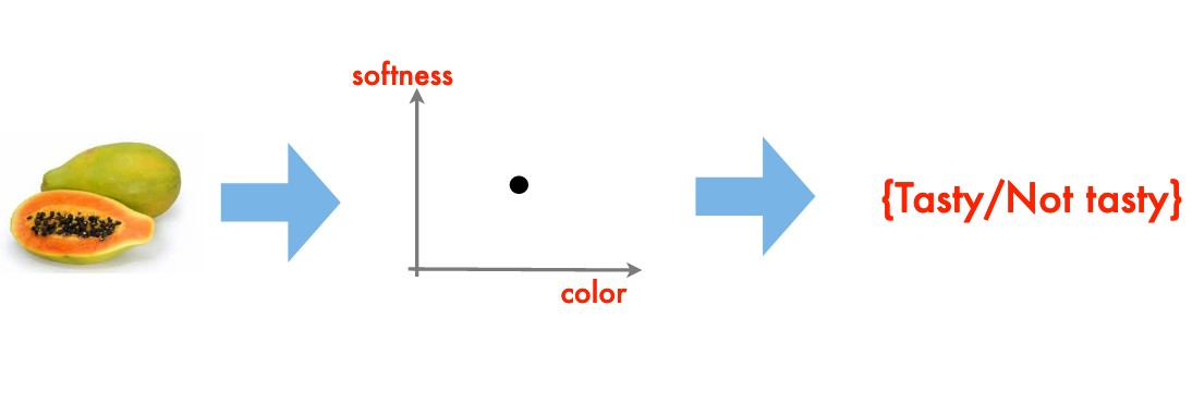
The resulting “rule” is a classification engine.

Note

I have implicitly assumed that there are quantitative metrics for softness and color (RGB+intensity perhaps), and we don’t want to actually put one into our mouth. An interesting twist on this example would be Durian, a most tasty fruit but in its harvested state most decidedly not soft nor of especially pleasing color.

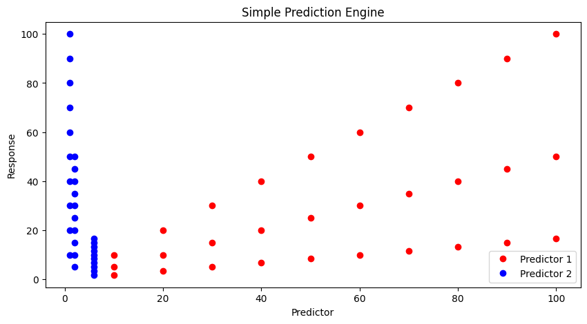
A Prediction Engine Example

Another simple example of machine learning (this time using numbers) is the mundane process of fitting a model to data; or in ML jargon the building of a prediction engine (the model equation) and subsequent application of the engine to new situations.

Consider a simple case where we have some observations like:

predictor1	predictor2	response
0.0	1.0	0.0
10.0	1.0	10.0
20.0	1.0	20.0
30.0	1.0	30.0
40.0	1.0	40.0
50.0	1.0	50.0
60.0	1.0	60.0
70.0	1.0	70.0
80.0	1.0	80.0
90.0	1.0	90.0
100.0	1.0	100.0
0.0	2.0	0.0
10.0	2.0	5.0
20.0	2.0	10.0
30.0	2.0	15.0
40.0	2.0	20.0
50.0	2.0	25.0
60.0	2.0	30.0
70.0	2.0	35.0
80.0	2.0	40.0
90.0	2.0	45.0
100.0	2.0	50.00
0.0	6.0	0.0
10.0	6.0	1.667
20.0	6.0	3.333
30.0	6.0	5.0
40.0	6.0	6.667
50.0	6.0	8.333
60.0	6.0	10.0
70.0	6.0	11.667
80.0	6.0	13.333
90.0	6.0	15.0
100.0	6.0	16.667

And if we simply try plotting we don’t learn much.

input1=[10.0,20.0,30.0,40.0,50.0,60.0,70.0,80.0,90.0,100.0,
        10.0,20.0,30.0,40.0,50.0,60.0,70.0,80.0,90.0,100.0,
        10.0,20.0,30.0,40.0,50.0,60.0,70.0,80.0,90.0,100.0,]
input2=[1.0,1.0,1.0,1.0,1.0,1.0,1.0,1.0,1.0,1.0,
        2.0,2.0,2.0,2.0,2.0,2.0,2.0,2.0,2.0,2.0,
        6.0,6.0,6.0,6.0,6.0,6.0,6.0,6.0,6.0,6.0]
output=[10.0,20.0,30.0,40.0,50.0,60.0,70.0,80.0,90.0,100.0,
        5.0,10.0,15.0,20.0,25.0,30.0,35.0,40.0,45.0,50.0, 
       1.6666833333333333, 3.3333666666666666, 5.00005, 6.666733333333333, 8.333416666666666, 10.0001, 11.666783333333331, 13.333466666666666, 15.00015, 16.666833333333333]

import matplotlib.pyplot as plt # the python plotting library
plottitle ='Simple Prediction Engine' 
mydata = plt.figure(figsize = (10,5)) # build a square drawing canvass from figure class
plt.plot(input1, output, c='red',linewidth=0,marker='o') 
plt.plot(input2, output, c='blue',linewidth=0,marker='o')
#plt.plot(time, accumulate, c='blue',drawstyle='steps') # step plot
plt.xlabel('Predictor')
plt.ylabel('Response')
plt.legend(['Predictor 1','Predictor 2'])
plt.title(plottitle)
plt.show()

Lets postulate a prediction engine structure as

\[r=\beta_1 p_1^{\beta_2} \cdot \beta_3 p_2^{\beta_4}\]

and try to pick values that make the model explain the data - here strictly by plotting.

First our prediction engine

def response(beta1,beta2,beta3,beta4,predictor1,predictor2):
    response = (beta1*predictor1**beta2)*(beta3*predictor2**beta4)
    return(response)

Now some way to guess model parameters (the betas) and plot our model response against the observed response. Here we choose to plot the observed values versus model values, if we find a good model, the line should plot as equal value line (45 degree line)

beta1 = 1
beta2 = 1
beta3 = 1
beta4 = 1

howmany = len(output)
modeloutput = [0 for i in range(howmany)]

for i in range(howmany):
    modeloutput[i]=response(beta1,beta2,beta3,beta4,input1[i],input2[i])
    
# now the plot
plottitle ='Simple Prediction Engine' 
mydata = plt.figure(figsize = (10,5)) # build a square drawing canvass from figure class
plt.plot(modeloutput, output, c='red',linewidth=1,marker='o') 
#plt.plot(input2, output, c='blue',linewidth=0,marker='o')
#plt.plot(time, accumulate, c='blue',drawstyle='steps') # step plot
plt.xlabel('Model Value')
plt.ylabel('Observed Value')
#plt.legend(['Predictor 1','Predictor 2'])
plt.title(plottitle)
plt.show()

Our first try is not too great. Lets change \(\beta_2\)

beta1 = 1
beta2 = 2
beta3 = 1
beta4 = 1

howmany = len(output)
modeloutput = [0 for i in range(howmany)]

for i in range(howmany):
    modeloutput[i]=response(beta1,beta2,beta3,beta4,input1[i],input2[i])
    
# now the plot
plottitle ='Simple Prediction Engine' 
mydata = plt.figure(figsize = (10,5)) # build a square drawing canvass from figure class
plt.plot(modeloutput, output, c='red',linewidth=1,marker='o') 
#plt.plot(input2, output, c='blue',linewidth=0,marker='o')
#plt.plot(time, accumulate, c='blue',drawstyle='steps') # step plot
plt.xlabel('Model Value')
plt.ylabel('Observed Value')
#plt.legend(['Predictor 1','Predictor 2'])
plt.title(plottitle)
plt.show()

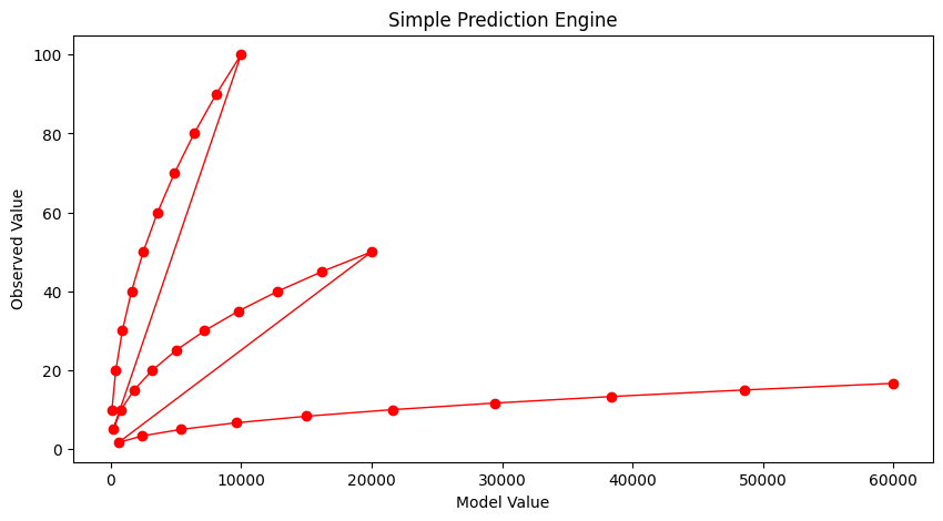
Not much help. After enough trials we might stumble on:

beta1 = 1
beta2 = 1
beta3 = 1
beta4 = -0.9

howmany = len(output)
modeloutput = [0 for i in range(howmany)]

for i in range(howmany):
    modeloutput[i]=response(beta1,beta2,beta3,beta4,input1[i],input2[i])
    
# now the plot
plottitle ='Simple Prediction Engine' 
mydata = plt.figure(figsize = (10,5)) # build a square drawing canvass from figure class
plt.plot(modeloutput, output, c='red',linewidth=1,marker='o') 
#plt.plot(input2, output, c='blue',linewidth=0,marker='o')
#plt.plot(time, accumulate, c='blue',drawstyle='steps') # step plot
plt.xlabel('Model Value')
plt.ylabel('Observed Value')
#plt.legend(['Predictor 1','Predictor 2'])
plt.title(plottitle)
plt.show()

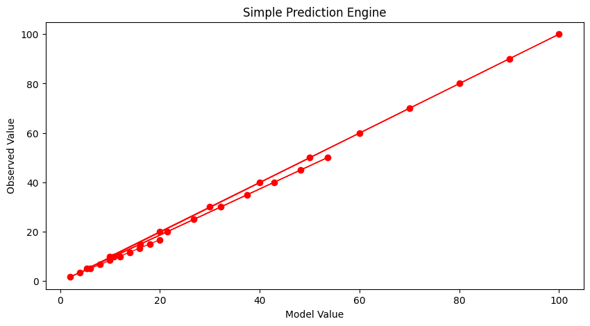
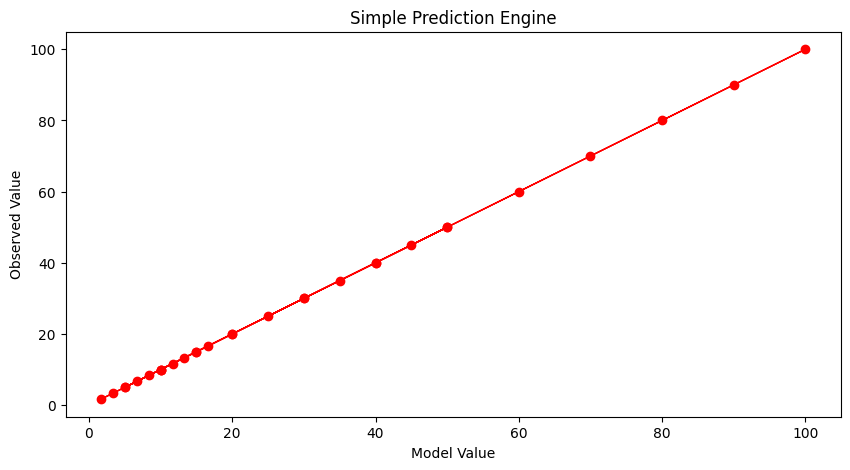
And that’s not too bad. What would help is some systematic way to automatically update the model parameters until we get a good enough prediction engine, then go out and use it. To get to perfection (which we can in this example because I know the data source), if we set the first three parameters to 1 and the last to -1 we obtain:

beta1 = 1
beta2 = 1
beta3 = 1
beta4 = -1

howmany = len(output)
modeloutput = [0 for i in range(howmany)]

for i in range(howmany):
    modeloutput[i]=response(beta1,beta2,beta3,beta4,input1[i],input2[i])
    
# now the plot
plottitle ='Simple Prediction Engine' 
mydata = plt.figure(figsize = (10,5)) # build a square drawing canvass from figure class
plt.plot(modeloutput, output, c='red',linewidth=1,marker='o') 
#plt.plot(input2, output, c='blue',linewidth=0,marker='o')
#plt.plot(time, accumulate, c='blue',drawstyle='steps') # step plot
plt.xlabel('Model Value')
plt.ylabel('Observed Value')
#plt.legend(['Predictor 1','Predictor 2'])
plt.title(plottitle)
plt.show()

Now with our machine all learned up we can use it for other cases, for instance if the inputs are [121,2]

print('predicted response is',response(beta1,beta2,beta3,beta4,121,2))

predicted response is 60.5

Automating the Process

To complete this example, instead of us (humans) doing the trial and error, lets let the machine do the work. For that we need a way to assess the ‘quality’ of our prediction model, a way to make new guesses, and a way to rank findings.

A terribly inefficient way, but easy to script is a grid search. We will take our 4 parameters and try combinations for values ranging between -1 and 1 and declare the best combination the model.

# identify, collect, load data

input1=[10.0,20.0,30.0,40.0,50.0,60.0,70.0,80.0,90.0,100.0,
        10.0,20.0,30.0,40.0,50.0,60.0,70.0,80.0,90.0,100.0,
        10.0,20.0,30.0,40.0,50.0,60.0,70.0,80.0,90.0,100.0,]
input2=[1.0,1.0,1.0,1.0,1.0,1.0,1.0,1.0,1.0,1.0,
        2.0,2.0,2.0,2.0,2.0,2.0,2.0,2.0,2.0,2.0,
        6.0,6.0,6.0,6.0,6.0,6.0,6.0,6.0,6.0,6.0]
output=[10.0,20.0,30.0,40.0,50.0,60.0,70.0,80.0,90.0,100.0,
        5.0,10.0,15.0,20.0,25.0,30.0,35.0,40.0,45.0,50.0, 
       1.6666833333333333, 3.3333666666666666, 5.00005, 6.666733333333333, 8.333416666666666, 10.0001, 11.666783333333331, 13.333466666666666, 15.00015, 16.666833333333333]

# a prediction engine structure (notice some logic to handle zeros)
def response(beta1,beta2,beta3,beta4,predictor1,predictor2):
    if predictor1 == 0.0 and predictor2 ==0.0:
        response = (beta1*predictor1**abs(beta2))*(beta3*predictor2**abs(beta4))
    if predictor1 == 0.0 and predictor2 !=0.0:
        response = (beta1*predictor1**abs(beta2))*(beta3*predictor2**(beta4))
    if predictor1 != 0.0 and predictor2 ==0.0:
        response = (beta1*predictor1**(beta2))*(beta3*predictor2**abs(beta4))
    if predictor1 != 0.0 and predictor2 !=0.0:
        response = (beta1*predictor1**(beta2))*(beta3*predictor2**(beta4))
    else:
        response = 1e9
    return(response)
# a measure of model quality
def quality(observed_list,model_list): 
    if len(observed_list) != len(model_list):
        raise Exception("List lengths incompatable")
    sse = 0.0
    howmany=len(observed_list)
    for i in range(howmany):
        sse=sse + (observed_list[i]-model_list[i])**2
    return(sse)
# define search region 
index_list = [i/10 for i in range(-20,21,2)] # index list is -1.0,-0.9,-0.8,....,0.9,1.0

howmany = 0 # keep count of how many combinations
error   = 1e99          # a big value, we are trying to drive this to zero
xbest   = [-1,-1,-1,-1] # variables to store our best solution parameters
modeloutput = [0 for i in range(len(output))] # space to store model responses


# perform a search - here we use nested repetition
for i1 in index_list:
    for i2 in index_list:
        for i3 in index_list:
            for i4 in index_list:
                howmany=howmany+1 # keep count of how many times we learn
                beta1 = i1
                beta2 = i2
                beta3 = i3
                beta4 = i4

                for irow in range(len(output)): 
                    modeloutput[irow]=response(beta1,beta2,beta3,beta4,input1[irow],input2[irow])
                guess = quality(output,modeloutput) # current model quality
 #               print(guess)
                if guess <= error:
                    error = guess
                    xbest[0]= beta1
                    xbest[1]= beta2
                    xbest[2]= beta3
                    xbest[3]= beta4
print("Search Complete - Error Value ",round(error,8))
print("Combinations Examined : ",howmany)
print("Beta 1 ",xbest[0])
print("Beta 2 ",xbest[1])
print("Beta 3 ",xbest[2])
print("Beta 4 ",xbest[3])
for irow in range(len(output)): 
    modeloutput[irow]=response(xbest[0],xbest[1],xbest[2],xbest[3],input1[irow],input2[irow])

# now the plot
import matplotlib.pyplot as plt # the python plotting library
plottitle ='Simple Prediction Engine - Automated Learning \n'
plottitle = plottitle + 'Model Error =' + repr(round(error,8)) + '\n'
plottitle = plottitle + 'Beta =' + repr(xbest)
mydata = plt.figure(figsize = (10,5)) # build a square drawing canvass from figure class
plt.plot(modeloutput, output, c='red',linewidth=1,marker='o') 
#plt.plot(input2, output, c='blue',linewidth=0,marker='o')
#plt.plot(time, accumulate, c='blue',drawstyle='steps') # step plot
plt.xlabel('Model Value')
plt.ylabel('Observed Value')
#plt.legend(['Predictor 1','Predictor 2'])
plt.title(plottitle)
plt.show()

Search Complete - Error Value  1.1e-07
Combinations Examined :  194481
Beta 1  1.0
Beta 2  1.0
Beta 3  1.0
Beta 4  -1.0

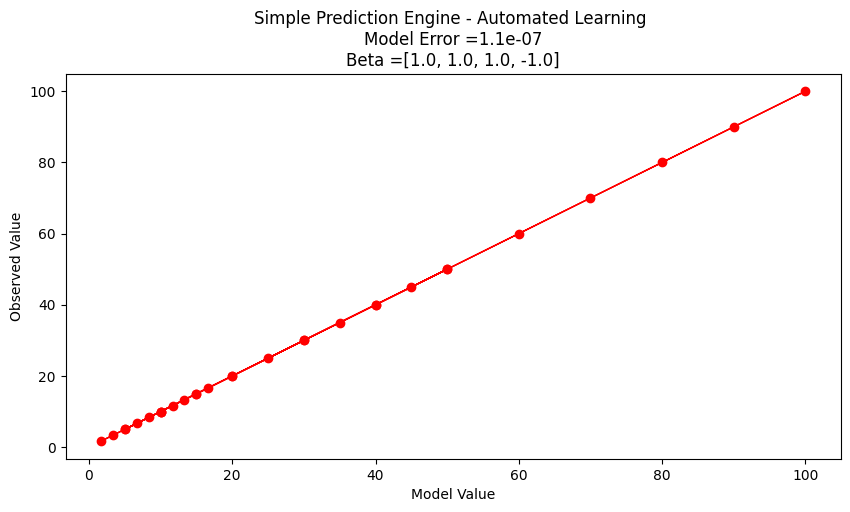
Interpreting our results

Suppose we are happy with the results, lets examine what the machine is telling us.

First if we examine the engine structure using the values fitted we have

• Our original structure before our engine got learned

\[r=\beta_1 p_1^{\beta_2} \cdot \beta_3 p_2^{\beta_4}\]

• After its all learned up!

\[r=1.0 p_1^{1.0} \cdot 1.0 p_2^{-1.0}\]

• Lets do a little algebra

\[r=\frac{p_1 }{p_2}\]

A little soul searching and we realize that \(\beta_1 \cdot \beta_3\) is really a single parameter and not really two different ones. If we knew that ahead of time, our seacrh region could be reduced. At this point all we really wanted here is an example of ML to produce a prediction engine (exclusive of the symbolic representation). We have done it the model is

\[r=\frac{p_1 }{p_2}\]

If we were to use it for future response prediction, then a user interface is in order. Something as simple as:

newp1 = 119
newp2 = 2.1
newot = response(xbest[0],xbest[1],xbest[2],xbest[3],newp1,newp2)
print('predicted response to predictor1 =',newp1,'and predictor2 =',newp2,' is :',round(newot,3))

predicted response to predictor1 = 119 and predictor2 = 2.1  is : 56.667

heading title

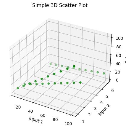
Before we exit this section lets examine the last example a bit more. We have a two-dimensional input structure, so we can conceivably plot the input space and the response into the 3-rd axis. First just the observations.

#!/usr/bin/python3

import sys
import matplotlib
import matplotlib.pyplot as plt
from mpl_toolkits.mplot3d import Axes3D

import numpy as np

# Input data
input1 = [10.0, 20.0, 30.0, 40.0, 50.0, 60.0, 70.0, 80.0, 90.0, 100.0,
          10.0, 20.0, 30.0, 40.0, 50.0, 60.0, 70.0, 80.0, 90.0, 100.0,
          10.0, 20.0, 30.0, 40.0, 50.0, 60.0, 70.0, 80.0, 90.0, 100.0]
input2 = [1.0, 1.0, 1.0, 1.0, 1.0, 1.0, 1.0, 1.0, 1.0, 1.0,
          2.0, 2.0, 2.0, 2.0, 2.0, 2.0, 2.0, 2.0, 2.0, 2.0,
          6.0, 6.0, 6.0, 6.0, 6.0, 6.0, 6.0, 6.0, 6.0, 6.0]
output = [10.0, 20.0, 30.0, 40.0, 50.0, 60.0, 70.0, 80.0, 90.0, 100.0,
          5.0, 10.0, 15.0, 20.0, 25.0, 30.0, 35.0, 40.0, 45.0, 50.0, 
          1.6666833333333333, 3.3333666666666666, 5.00005, 6.666733333333333, 8.333416666666666, 10.0001, 11.666783333333331, 13.333466666666666, 15.00015, 16.666833333333333]

# Combine inputs into a single dataset
DATA = np.array(list(zip(input1, input2, output)))

Xs = DATA[:, 0]
Ys = DATA[:, 1]
Zs = DATA[:, 2]

# Creating figure
fig = plt.figure(figsize=(5, 5))
ax = plt.axes(projection="3d")

# Creating plot
ax.scatter3D(Xs, Ys, Zs, color="green")
plt.title("Simple 3D Scatter Plot")
plt.xlabel("Input 1")
plt.ylabel("Input 2")
ax.set_zlabel("Output")

# Show plot
plt.show()

Assuming the response is some smooth function of the input feature values, we could attempt a contour plot.

import pandas
my_xyz = pandas.DataFrame(DATA) # convert into a data frame
import numpy 
import matplotlib.pyplot
from scipy.interpolate import griddata
# extract lists from the dataframe
coord_x = my_xyz[0].values.tolist()
coord_y = my_xyz[1].values.tolist()
coord_z = my_xyz[2].values.tolist()
coord_xy = numpy.column_stack((coord_x, coord_y))
# Set plotting range in original data units
lon = numpy.linspace(min(coord_x), max(coord_x), 300)
lat = numpy.linspace(min(coord_y), max(coord_y), 300)
X, Y = numpy.meshgrid(lon, lat)
# Grid the data; use cubic spline interpolation (other choices are nearest and linear)
Z = griddata(numpy.array(coord_xy), numpy.array(coord_z), (X, Y), method='linear', fill_value = 'nan')
# Build the map
matplotlib.pyplot.rcParams["figure.figsize"] = [12.00, 6.00]
matplotlib.pyplot.rcParams["figure.autolayout"] = True
fig, ax = matplotlib.pyplot.subplots()
levels=[5,10,15,20,25,30,35,40,45,50]
CS = ax.contour(X, Y, Z, levels=20, linewidths=3)
ax.plot([50,50],[0,7])
ax.plot([10,100],[5,5])
ax.plot(coord_x,coord_y,marker=".",linestyle="none",markersize=13)
ax.clabel(CS, inline=2, fontsize=12)
ax.set_title('Contour Plot from Gridded Data File')
ax.set_xlim([0,120])
ax.set_ylim([0,7]);

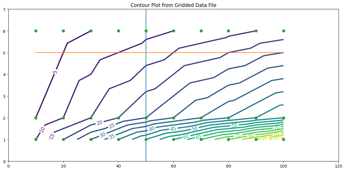
We could use this as the predcition engine - for instance the plot suggests that at (50,5) the response should be between 10 and 15 (based on the plotted contours); notice (50,5) is NOT in the observation set - so this is truely a prediction.

Note

A graphical representation of complex behavior was the standard of communication and prediction tools for centuries - they are only now being replaced with computed predictions because the hardware and software are now capable and affordable.

newp1 = 50
newp2 = 5
newot = response(xbest[0],xbest[1],xbest[2],xbest[3],newp1,newp2)
print('predicted response to predictor1 =',newp1,'and predictor2 =',newp2,' is :',round(newot,3))

predicted response to predictor1 = 50 and predictor2 = 5  is : 10.0

So whats going on with the prediction? The contour plot has an implied data model (probably inverse distance - we would need to look at the internals of the gridding tool); our ML model has a different implied data model - we really don’t know which one is better until we get a new observation, then in either case we would rerun the “training step” to update the model.

Now notice something our ML model can do that our contour plot does not do (easily) - that is to extrapolate beyond the input ranges smoothly.

For instance at (110,3) the contour plot shows us nothing at best the response will be in the 20s to 30s if we mentally extend the contour lines. To the ML model its just another input/response combination:

newp1 = 110
newp2 = 3
newot = response(xbest[0],xbest[1],xbest[2],xbest[3],newp1,newp2)
print('predicted response to predictor1 =',newp1,'and predictor2 =',newp2,' is :',round(newot,3))

predicted response to predictor1 = 110 and predictor2 = 3  is : 36.667

So that’s an elementary prediction engine, ML example - all pretty much homebrew, with some interpretation. It is crude but does capture the essence of ML. We constructed a function to assess how close a computed prediction came to an observation (our merit function); we decided that making the function small was good (our goal to seek); and we developed a way to update the weights embedded in the prediction function (our optimization function). Later on we will see that these characteristics are in some fashion shared by all ML tools.

A classification example is saved for another lesson, but it too will have these essential characteristics.

Learning Types

Three broad classifications of ML are described below.

Supervised Learning

Supervised learning is a machine learning approach where the algorithm learns to map inputs to desired outputs using labeled training data. Each example in the dataset contains an input-output pair, allowing the model to learn patterns and relationships.

• How It Works: The algorithm iteratively adjusts its parameters to minimize the error between predicted outputs and the true outputs. Common techniques include regression for continuous outputs and classification for discrete outputs.

• Example: Predicting housing prices based on features like square footage, number of bedrooms, and location. The dataset includes both the features (inputs) and the actual sale prices (outputs).

Unsupervised Learning

Unsupervised learning involves training algorithms on datasets without labeled outputs. The goal is to identify hidden structures, patterns, or clusters in the data.

• How It Works: The model analyzes data to uncover similarities or anomalies without any explicit supervision. Popular methods include clustering (e.g., k-means) and dimensionality reduction (e.g., PCA).

• Example: Grouping customers based on purchasing behavior to tailor marketing strategies. The algorithm clusters customers into segments without prior knowledge of their identities or preferences.

Reinforcement Learning

Reinforcement learning focuses on training agents to make decisions by interacting with an environment. The agent learns by trial and error, receiving rewards or penalties based on its actions.

• How It Works: The agent’s goal is to maximize cumulative rewards by learning an optimal policy—a sequence of actions that leads to the best outcomes. Key components include states, actions, rewards, and policies.

• Example: Training a robot to navigate a maze. The robot receives positive rewards for reaching the exit and negative rewards for hitting walls, learning an effective path over time.

Machine Learning Workflow

Despite the diverse applications of machine learning, most machine learning projects follow a typical workflow. Prior to examination of workflow consider ordinary problem solving.

Computational Thinking and Data Science

Computational thinking (CT) refers to the thought processes involved in expressing solutions as computational steps or algorithms that can be carried out by a computer.

CT is literally a process for breaking down a problem into smaller parts, looking for patterns in the problems, identifying what kind of information is needed, developing a step-by-step solution, and implementing that solution.

1. Decomposition is the process of taking a complex problem and breaking it into more manageable sub-problems. Decomposition often leaves a framework of sub-problems that later have to be assembled (system integration) to produce a desired solution.

2. Pattern Recognition refers to finding similarities, or shared characteristics of problems, which allows a complex problem to become easier to solve, and allows use of same solution method for each occurrence of the pattern.

3. Abstraction is the process of identifying important characteristics of the problem and ignore characteristics that are not important. We use these characteristics to create a representation of what we are trying to solve.

4. Algorithms are step-by-step instructions of how to solve a problem

5. System Integration (implementation)is the assembly of the parts above into the complete (integrated) solution. Integration combines parts into a program which is the realization of an algorithm using a syntax that the computer can understand.

Problem Solving Protocol

Many engineering courses emphasize a problem solving process that somewhat parallels the scientific method as one example of an effective problem solving strategy. Stated as a protocol it goes something like:

1. Observation: Formulation of a question

2. Hypothesis: A conjecture that may explain observed behavior. Falsifiable by an experiment whose outcome conflicts with predictions deduced from the hypothesis

3. Prediction: How the experiment should conclude if hypothesis is correct

4. Testing: Experimental design, and conduct of the experiment.

5. Analysis: Interpretation of experimental results

This protocol can be directly adapted to computational problems as:

1. Define the problem (problem statement)

2. Gather information (identify known and unknown values, and governing equations)

3. Generate and evaluate potential solutions

4. Refine and implement a solution

5. Verify and test the solution.

For actual computational methods the protocol becomes:

1. Explicitly state the problem

2. State:

• Input information

• Governing equations or principles, and

• The required output information.

3. Work a sample problem by-hand for testing the general solution.

4. Develop a general solution method (coding).

5. Test the general solution against the by-hand example, then apply to the real problem.

Oddly enough the first step is the most important and sometimes the most difficult. In a practical problem, step 2 is sometimes difficult because a skilled programmer is needed to translate the governing principles into an algorithm for the general solution (step 4).

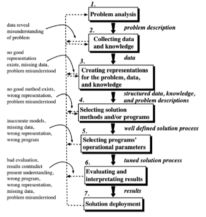
We can compare the steps above to a visual representation of the process below from Machine Learning Techniques for Civil Engineering Problems.

ML Workflow Steps

A typical machine learning workflow includes some (or all) of the steps listed below adapted from Machine Learning With Python For Beginners. As you examine the steps compare them to the more classical problem solving approaches to recognize the parallels.

• Step 1. Identify, Collect, and Loading Data. (Data Wrangling) The first step to any machine learning project is to load the data. Based on the data at hand, we would need different libraries to load the respective data. If we are using a python derivative to perform the modeling then for loading CSV files, we need the pandas library. For loading 2D images, we can use the Pillow or OpenCV library.

• Step 2. Examine the data. (Exploratory Data Analysis) Assuming the data has been loaded correctly, the next step is to examine the data to get a general feel for the dataset. Let us take the case of a simple CSV file-based dataset. For starters, we can look at the dataset’s shape (i.e., the number of rows and columns in the dataset). We can also peek inside the dataset by looking at its first 10 or 20 rows. In addition, we can perform fundamental analysis on the data to generate some descriptive statistical measures (such as the mean, standard deviation, minimum and maximum values). Last but not least, we can check if the dataset contains missing data. If there are missing values, we need to handle them.

• Step 3. Split the Dataset. (Training and Testing Subsets) Before we handle missing values or do any form of computation on our dataset, we typically typically split it into training and test subsets. A common practice is to use 80% of the dataset for training and 20% for testing although the proportions are up to the program designer. The training subset is the actual dataset used for training the model. After the training process is complete, we can use the test subset to evaluate how well the model generalizes to unseen data (i.e., data not used to train the model). It is crucial to treat the test subset as if it does not exist during the training stage. Therefore, we should not touch it until we have finished training our model and are ready to evaluate the selected model.

Note

A huge philosophical issue arises if the testing set suggests that we have a crappy model - at that juncture if we change the model at all the testing set has just been used for training and calls into question the whole split data process. This dilemma is rarely discussed in the literature, but is an important ethical issue to keep in mind when letting a machine control things that can kill. Most people think hellfire missles and drones, but water treatment plants under unattended autonomous control can kill as effectively as a missle.

• Step 4. Data Visualization (Exploratory Data Analysis) After splitting the dataset, we can plot some graphs to better understand the data we are investigating. For instance, we can plot scatter plots to investigate the relationships between the features (explainatory variables, predictor variables, etc.) and the target (response) variable.

• Step 5. Data Preprocessing. (Data Structuring) The next step is to do data preprocessing. More often than not, the data that we receive is not ready to be used immediately. Some problems with the dataset include missing values, textual and categorical data (e.g., “Red”, “Green”, and “Blue” for color), or range of features that differ too much (such as a feature with a range of 0 to 10,000 and another with a range of 0 to 5). Most machine learning algorithms do not perform well when any of the issues above exist in the dataset. Therefore, we need to process the data before passing it to the algorithm.

• Step 6. Model Training. After preparing the data, we are ready to train our models. Based on the previous steps of analyzing the dataset, we can select appropriate machine learning algorithms and build models using those algorithms.

• Step 7. Performance Evaluation. After building the models, we need to evaluate our models using different metrics and select the best-performing model for deployment. At this stage, the technical aspects of a machine learning project is more or less complete.

• Step 8. Deploy the Model. Deploy the best-performing model. Build a user interface so customers/designers/clients can apply the model to their needs.

• Step 9. Monitoring and maintaining the model. This step is quite overlooked in most documents on ML, even more so than deploy. This step would audit post-deployment use and from time-to-time re-train the model with newer data. Some industries perform this retraining almost continuously; in Civil Engineering the retraining may happen on a decade-long time scale perhaps even longer. It depends on the consequence of failure, and the model value.

Consider the Figure below as another representation of workflow from Machine Learning Workflow Explained.

ML Workflow Diagram

The figure components largely address each list item, some are shared, others combined - nevertheless we have a suitable workflow diagram. The author of the diagram places data at the top and cycles from there, a subtle symbolic placement with which I wholly agree. Read his blog post to see his thinking in that respect.

Anatomy of a Machine Learning Algorithm

The fundamental building blocks of a ML algorithm, whether homebrew or using a package consist of three major components:

1. a function to assess the quality of a prediction or classification. Typically a loss function which we want to minimize, or a likelihood function which we want to maximize. It goes by many names: objective, cost, loss, merit are common names for this function.

2. an objective criterion (a goal) based on the loss function (maximize or minimize), and

3. an optimization routine that uses the training data to find a solution to the optimization problem posed by the objective criterion.

The remainder of this Jupyter Book explores these ideas as well as supporting efforts required for useful ML model building for Civil Engineers (actually anyone).

End of Section