Hooke and Jeeves Pattern Search#
The Hooke and Jeeves algorithm is a classic pattern search method for nonlinear optimization, particularly suited for problems where derivative information is unavailable or unreliable.
This method alternates between two key steps:
Exploratory moves that test directions along coordinate axes.
Pattern moves that use momentum from successful steps to accelerate progress.
It is a derivative-free method, making it well suited for:
Black-box functions
Discontinuous or noisy objective landscapes
Engineering problems where gradients are hard to compute
References#
Videos#
The hookeNjeeves module#
The optimization logic is implemented in a Python module, hookeNjeeves.py.
Hooke and Jeeves Search Module Code
# Hooke and Jeeves Search as python script for import into Jupyter
# Minimal Script.
#
#     This is a direct python port of Mark G. Johnson's C implementation of the Hooke and Jeeves algorithm
#
#     Sean R. Johnson, July 7, 2013
#
#     immediately below is the original documentation
#     in the body, comments marked with ## are from the original,
#     other comments are my own
#

#/* Nonlinear Optimization using the algorithm of Hooke and Jeeves  */
#/*	12 February 1994	author: Mark G. Johnson 	   */

#/* Find a point X where the nonlinear function f(X) has a local    */
#/* minimum.  X is an n-vector and f(X) is a scalar.  In mathe-	   */
#/* matical notation  f: R^n -> R^1.  The objective function f()    */
#/* is not required to be continuous.  Nor does f() need to be	   */
#/* differentiable.  The program does not use or require 	   */
#/* derivatives of f().						   */

#/* The software user supplies three things: a subroutine that	   */
#/* computes f(X), an initial "starting guess" of the minimum point */
#/* X, and values for the algorithm convergence parameters.  Then   */
#/* the program searches for a local minimum, beginning from the    */
#/* starting guess, using the Direct Search algorithm of Hooke and  */
#/* Jeeves.							   */

#/* This C program is adapted from the Algol pseudocode found in    */
#/* "Algorithm 178: Direct Search" by Arthur F. Kaupe Jr., Commun-  */
#/* ications of the ACM, Vol 6. p.313 (June 1963).  It includes the */
#/* improvements suggested by Bell and Pike (CACM v.9, p. 684, Sept */
#/* 1966) and those of Tomlin and Smith, "Remark on Algorithm 178"  */
#/* (CACM v.12).  The original paper, which I don't recommend as    */
#/* highly as the one by A. Kaupe, is:  R. Hooke and T. A. Jeeves,  */
#/* "Direct Search Solution of Numerical and Statistical Problems", */
#/* Journal of the ACM, Vol. 8, April 1961, pp. 212-229. 	   */

#/* Calling sequence:						   */
#/*  int hooke(nvars, startpt, endpt, rho, epsilon, itermax)	   */
#/*								   */
#/*     nvars	   {an integer}  This is the number of dimensions  */
#/*		   in the domain of f().  It is the number of	   */
#/*		   coordinates of the starting point (and the	   */
#/*		   minimum point.)				   */
#/*     startpt	   {an array of doubles}  This is the user-	   */
#/*		   supplied guess at the minimum.		   */
#/*     endpt	   {an array of doubles}  This is the location of  */
#/*		   the local minimum, calculated by the program    */
#/*     rho	   {a double}  This is a user-supplied convergence */
#/*		   parameter (more detail below), which should be  */
#/*		   set to a value between 0.0 and 1.0.	Larger	   */
#/*		   values of rho give greater probability of	   */
#/*		   convergence on highly nonlinear functions, at a */
#/*		   cost of more function evaluations.  Smaller	   */
#/*		   values of rho reduces the number of evaluations */
#/*		   (and the program running time), but increases   */
#/*		   the risk of nonconvergence.	See below.	   */
#/*     epsilon	   {a double}  This is the criterion for halting   */
#/*		   the search for a minimum.  When the algorithm   */
#/*		   begins to make less and less progress on each   */
#/*		   iteration, it checks the halting criterion: if  */
#/*		   the stepsize is below epsilon, terminate the    */
#/*		   iteration and return the current best estimate  */
#/*		   of the minimum.  Larger values of epsilon (such */
#/*		   as 1.0e-4) give quicker running time, but a	   */
#/*		   less accurate estimate of the minimum.  Smaller */
#/*		   values of epsilon (such as 1.0e-7) give longer  */
#/*		   running time, but a more accurate estimate of   */
#/*		   the minimum. 				   */
#/*     itermax	   {an integer}  A second, rarely used, halting    */
#/*		   criterion.  If the algorithm uses >= itermax    */
#/*		   iterations, halt.				   */


#/* The user-supplied objective function f(x,n) should return a C   */
#/* "double".  Its  arguments are  x -- an array of doubles, and    */
#/* n -- an integer.  x is the point at which f(x) should be	   */
#/* evaluated, and n is the number of coordinates of x.	That is,   */
#/* n is the number of coefficients being fitted.		   */

#/* rho, the algorithm convergence control			   */
#/*	The algorithm works by taking "steps" from one estimate of */
#/*    a minimum, to another (hopefully better) estimate.  Taking   */
#/*    big steps gets to the minimum more quickly, at the risk of   */
#/*    "stepping right over" an excellent point.  The stepsize is   */
#/*    controlled by a user supplied parameter called rho.  At each */
#/*    iteration, the stepsize is multiplied by rho  (0 < rho < 1), */
#/*    so the stepsize is successively reduced.			   */
#/*	Small values of rho correspond to big stepsize changes,    */
#/*    which make the algorithm run more quickly.  However, there   */
#/*    is a chance (especially with highly nonlinear functions)	   */
#/*    that these big changes will accidentally overlook a	   */
#/*    promising search vector, leading to nonconvergence.	   */
#/*	Large values of rho correspond to small stepsize changes,  */
#/*    which force the algorithm to carefully examine nearby points */
#/*    instead of optimistically forging ahead.	This improves the  */
#/*    probability of convergence.				   */
#/*	The stepsize is reduced until it is equal to (or smaller   */
#/*    than) epsilon.  So the number of iterations performed by	   */
#/*    Hooke-Jeeves is determined by rho and epsilon:		   */
#/*	    rho**(number_of_iterations) = epsilon		   */
#/*	In general it is a good idea to set rho to an aggressively */
#/*    small value like 0.5 (hoping for fast convergence).  Then,   */
#/*    if the user suspects that the reported minimum is incorrect  */
#/*    (or perhaps not accurate enough), the program can be run	   */
#/*    again with a larger value of rho such as 0.85, using the	   */
#/*    result of the first minimization as the starting guess to    */
#/*    begin the second minimization.				   */

#/* Normal use: (1) Code your function f() in the C language	   */
#/*	       (2) Install your starting guess {or read it in}	   */
#/*	       (3) Run the program				   */
#/*	       (4) {for the skeptical}: Use the computed minimum   */
#/*		      as the starting point for another run	   */

#/* Data Fitting:						   */
#/*	Code your function f() to be the sum of the squares of the */
#/*	errors (differences) between the computed values and the   */
#/*	measured values.  Then minimize f() using Hooke-Jeeves.    */
#/*	EXAMPLE: you have 20 datapoints (ti, yi) and you want to   */
#/*	find A,B,C such that  (A*t*t) + (B*exp(t)) + (C*tan(t))    */
#/*	fits the data as closely as possible.  Then f() is just    */
#/*	f(x) = SUM (measured_y[i] - ((A*t[i]*t[i]) + (B*exp(t[i])) */
#/*				  + (C*tan(t[i]))))^2		   */
#/*	where x[] is a 3-vector consisting of {A, B, C}.	   */

#/*								   */
#/*  The author of this software is M.G. Johnson.		   */
#/*  Permission to use, copy, modify, and distribute this software  */
#/*  for any purpose without fee is hereby granted, provided that   */
#/*  this entire notice is included in all copies of any software   */
#/*  which is or includes a copy or modification of this software   */
#/*  and in all copies of the supporting documentation for such	   */
#/*  software.  THIS SOFTWARE IS BEING PROVIDED "AS IS", WITHOUT    */
#/*  ANY EXPRESS OR IMPLIED WARRANTY.  IN PARTICULAR, NEITHER THE   */
#/*  AUTHOR NOR AT&T MAKE ANY REPRESENTATION OR WARRANTY OF ANY	   */
#/*  KIND CONCERNING THE MERCHANTABILITY OF THIS SOFTWARE OR ITS    */
#/*  FITNESS FOR ANY PARTICULAR PURPOSE. 			   */
#/*								   */
#import sys #you may need to activate on your computer

#def rosenbrock(x): # a classic example function - deactivated here and moved to actual call
#    '''
#        ## Rosenbrocks classic parabolic valley ("banana") function
#    '''
#    a = x[0]
#    b = x[1]
#    return ((1.0 - a)**2) + (100.0 * (b - (a**2))**2)

def _hooke_best_nearby(f, delta, point, prevbest, bounds=None, args=[]):
    '''
        ## given a point, look for a better one nearby
        one coord at a time

        f is a function that takes a list of floats (of the same length as point) as an input
        args is a dict of any additional arguments to pass to f
        delta, and point are same-length lists of floats
        prevbest is a float

        point and delta are both modified by the function
    '''
    z = [x for x in point]
    minf = prevbest
    ftmp = 0.0

    fev = 0

    for i in range(len(point)):
        #see if moving point in the positive delta direction decreases the
        z[i] = _value_in_bounds(point[i] + delta[i], bounds[i][0], bounds[i][1])

        ftmp = f(z, *args)
        fev += 1
        if ftmp < minf:
            minf = ftmp
        else:
            #if not, try moving it in the other direction
            delta[i] = -delta[i]
            z[i] = _value_in_bounds(point[i] + delta[i], bounds[i][0], bounds[i][1])

            ftmp = f(z, *args)
            fev += 1
            if ftmp < minf:
                minf = ftmp
            else:
#if moving the point in both delta directions result in no improvement, then just keep the point where it is
                z[i] = point[i]

    for i in range(len(z)):
        point[i] = z[i]
    return (minf, fev)

def _point_in_bounds(point, bounds):
    '''
        shifts the point so it is within the given bounds
    '''
    for i in range(len(point)):
        if point[i] < bounds[i][0]:
            point[i] = bounds[i][0]
        elif point[i] > bounds[i][1]:
            point[i] = bounds[i][1]

def _is_point_in_bounds(point, bounds):
    '''
        true if the point is in the bounds, else false
    '''
    out = True
    for i in range(len(point)):
        if point[i] < bounds[i][0]:
            out = False
        elif point[i] > bounds[i][1]:
            out = False
    return out

def _value_in_bounds(val, low, high):
    if val < low:
        return low
    elif val > high:
        return hight
    else:
        return val

def hooke(f, startpt, bounds=None, rho=0.5, epsilon=1E-6, itermax=5000, args=[]):
#
    '''
    In this version of the Hooke and Jeeves algorithm, we coerce the function into staying within the given bounds.
    basically, any time the function tries to pick a point outside the bounds we shift the point to the boundary
    on whatever dimension it is out of bounds in. Implementing bounds this way may be questionable from a theory standpoint,
    but that's how COPASI does it, that's how I'll do it too.

    '''

    result = dict()
    result['success'] = True
    result['message'] = 'success'

    delta = [0.0] * len(startpt)
    endpt = [0.0] * len(startpt)
    if bounds is None:
        # if bounds is none, make it none for all (it will be converted to below)
        bounds = [[None,None] for x in startpt]
    else:
        bounds = [[x[0],x[1]] for x in bounds] #make it so it wont update the original
    startpt = [x for x in startpt] #make it so it wont update the original

    fmin = None
    nfev = 0
    iters = 0

    for bound in bounds:
        if bound[0] is None:
            bound[0] = float('-inf')
        else:
            bound[0] = float(bound[0])
        if bound[1] is None:
            bound[1] = float('inf')
        else:
            bound[1] = float(bound[1])
    try:
        # shift
        _point_in_bounds(startpt, bounds) #shift startpt so it is within the bounds

        xbefore = [x for x in startpt]
        newx = [x for x in startpt]
        for i in range(len(startpt)):
            delta[i] = abs(startpt[i] * rho)
            if (delta[i] == 0.0):
                # we always want a non-zero delta because otherwise we'd just be checking the same point over and over
                # and wouldn't find a minimum
                delta[i] = rho

        steplength = rho

        fbefore = f(newx, *args)
        nfev += 1

        newf = fbefore
        fmin = newf
        while ((iters < itermax) and (steplength > epsilon)):
            iters += 1
            #print "after %5d , f(x) = %.4le at" % (funevals, fbefore)

#        for j in range(len(startpt)):
#            print "   x[%2d] = %4le" % (j, xbefore[j])
#            pass

###/* find best new point, one coord at a time */
            newx = [x for x in xbefore]
            (newf, evals) = _hooke_best_nearby(f, delta, newx, fbefore, bounds, args)

            nfev += evals
###/* if we made some improvements, pursue that direction */
            keep = 1
            while ((newf < fbefore) and (keep == 1)):
                fmin = newf
                for i in range(len(startpt)):
###/* firstly, arrange the sign of delta[] */
                    if newx[i] <= xbefore[i]:
                        delta[i] = -abs(delta[i])
                    else:
                        delta[i] = abs(delta[i])
## #/* now, move further in this direction */
                    tmp = xbefore[i]
                    xbefore[i] = newx[i]
                    newx[i] = _value_in_bounds(newx[i] + newx[i] - tmp, bounds[i][0], bounds[i][1])
                fbefore = newf
                (newf, evals) = _hooke_best_nearby(f, delta, newx, fbefore, bounds, args)
                nfev += evals
###/* if the further (optimistic) move was bad.... */
                if (newf >= fbefore):
                    break

## #/* make sure that the differences between the new */
## #/* and the old points are due to actual */
## #/* displacements; beware of roundoff errors that */
## #/* might cause newf < fbefore */
                keep = 0
                for i in range(len(startpt)):
                    keep = 1
                    if ( abs(newx[i] - xbefore[i]) > (0.5 * abs(delta[i])) ):
                        break
                    else:
                        keep = 0
            if ((steplength >= epsilon) and (newf >= fbefore)):
                steplength = steplength * rho
                delta = [x * rho for x in delta]
        for x in range(len(xbefore)):
            endpt[x] = xbefore[x]
    except Exception as e:
        exc_type, exc_obj, exc_tb = sys.exc_info()
        result['success'] = False
        result['message'] = str(e) + ". line number: " + str(exc_tb.tb_lineno)
    finally:
        result['nit'] = iters
        result['fevals'] = nfev
        result['fun'] = fmin
        result['x'] = endpt

    return result
This module defines the pattern search behavior and allows us to easily apply it to new problems by supplying:
An objective function
An initial guess
A step size
A shrink factor
A tolerance
The next cell demonstrates the module in use with a classic optimization benchmark.
Example 1: Rosenbrock Function#
The Rosenbrock function, also known as the banana function, is a standard test case in optimization. Its curved, narrow valley challenges many optimization methods.
The function is defined as:
A contour plot in the search range is
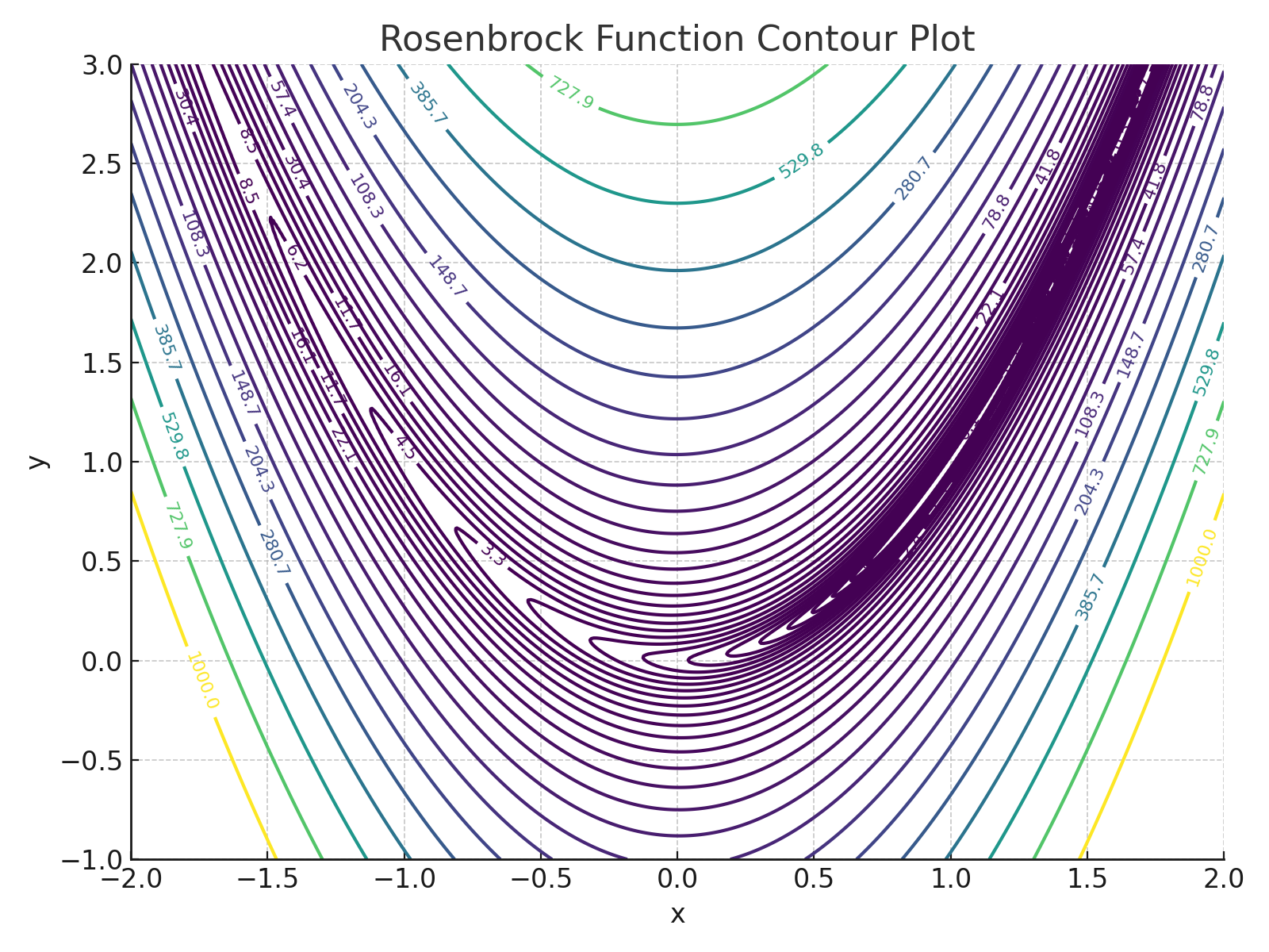
The function has a global minimum at \((x, y) = (1, 1)\), where \(f(x, y) = 0\).
Let’s use Hooke and Jeeves to find the minimum without using gradients.
import hookeNjeeves # import the script below from local file hookeNjeeves.py

def rosenbrock(x):
    '''
    Rosenbrock's classic parabolic valley ("banana") function.
    '''
    return (1 - x[0])**2 + 100 * (x[1] - x[0]**2)**2


bounds=[[-2, 2], [-1, 3]]  # Upper/Lower bounds
start = [-1.0,2.12]        # Initial guess
rho = 0.25                 # Step size change rate
epsilon = 1.0e-9           # Convergence threshold
itermax = 50               # Maximum iterations

print("Initial Objective Value :",rosenbrock(start))
res = hookeNjeeves.hooke(rosenbrock, start, bounds, rho, epsilon, itermax) # unconstrained
#print(res)
print("Minimum Value        :",res['fun'])
print("Optimum at           :",res['x'])
print("Function evaluations :", res['fevals'])
print("Number of Iterations :", res['nit'])
Initial Objective Value : 129.44
Minimum Value        : 1.802202459302945e-14
Optimum at           : [1.0000001341104507, 1.0000002676174993]
Function evaluations : 1870
Number of Iterations : 14
Hooke and Jeeves Search Process#
The search proceeds as follows:
Start at an initial guess \( x_0 \)
Perform exploratory search by evaluating function values in each coordinate direction.
If an improvement is found, take a pattern move in that direction.
If no improvement, reduce the step size.
Repeat until convergence criteria are met (e.g., small step size or no improvement).
Advantages:
Simple and intuitive
No derivatives needed
Flexible for arbitrary constraints or black-box evaluations
Disadvantages:
Slower than gradient-based methods in smooth problems
Sensitive to step size and shrink factor
Discussion Questions#
How did the search perform on the Rosenbrock function?
How would you tune the step size and shrink factor for better performance?
What kinds of problems might benefit from a Hooke and Jeeves approach in your domain?
Try It!#
Try using this same pattern search on a custom function — perhaps one from your design or lab work!