8. Decision Trees#
Course Website
lorem ipsum
Readings/References#
Burkov, A. (2019) The One Hundred Page Machine Learning Book Required Textbook
Rashid, Tariq. (2016) Make Your Own Neural Network. Kindle Edition. Required Textbook
United States Army Medical Command (MEDCOM) Algorithm Directed Troop Medical Care (ADTMC) manual
Chan, Jamie. Machine Learning With Python For Beginners: A Step-By-Step Guide with Hands-On Projects (Learn Coding Fast with Hands-On Project Book 7) (p. 2). Kindle Edition.
In-Depth: Decision Trees and Random Forests” by Jake VanderPlas
Powerful Guide to learn Random Forest (with codes in R & Python)” by SUNIL RAY
Introduction to Random forest – Simplified” by TAVISH SRIVASTAVA
“Random Forest Algorithm with Python and Scikit-Learn” by Usman Malik
AMOSIST Program Field Evaluation - DTIC Defense Technical Information Center (c. 1979) The US Army ‘s AMOSIST Program employed physician supervised enlisted corpsmen who utilize a manual of medical algorithms to provide care to troops in clinical and austere settings.
Asquith, W.H., and Roussel, M.C., 2007, An initial-abstraction, constant-loss model for unit hydrograph modeling for applicable watersheds in Texas: U.S. Geological Survey Scientific Investigations Report 2007–5243, 82 p. [ http://pubs.usgs.gov/sir/2007/5243 ] A hydrology model, that uses decision trees to parameterize the parts of the model. Example of a deployed model.
Videos#
“Decision Tree (CART) - Machine Learning Fun and Easy” by Augmented Startups
“StatQuest: Random Forests Part 1 - Building, Using and Evaluating” by StatQuest with Josh Starmer
“StatQuest: Random Forests Part 2: Missing data and clustering” by StatQuest with Josh Starmer
“Random Forest - Fun and Easy Machine Learning” by Augmented Startups
Background#
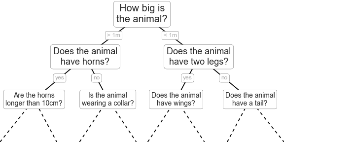
Classification And Regression Tree (CART) models, are intuitive ways to classify or label objects: you simply ask a series of questions designed to zero-in on the classification. For example, if you wanted to build a decision tree to classify an animal you come across while on a hike, you might construct the one shown here:
The binary splitting makes this extremely efficient: in a well-constructed tree, each question will cut the number of options by approximately half, very quickly narrowing the options even among a large number of classes. The trick, of course, comes in deciding which questions to ask at each step. In machine learning implementations of decision trees, the questions generally take the form of axis-aligned splits in the data: that is, each node in the tree splits the data into two groups using a cutoff value within one of the features. Let’s now look at an example of this.
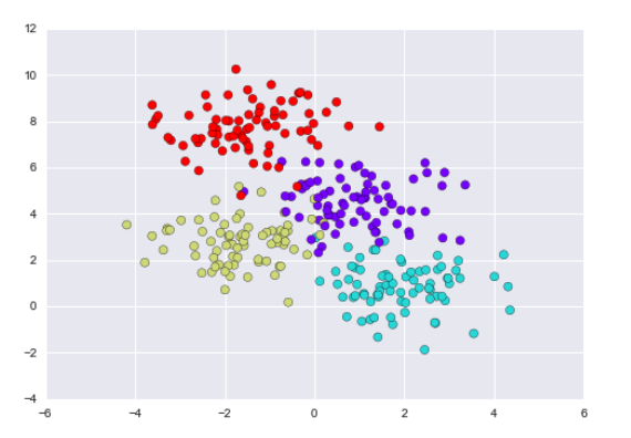
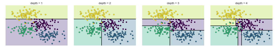
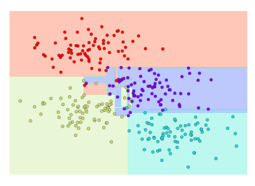
A simple decision tree built on this data will iteratively split the data along one or the other axis according to some quantitative criterion, and at each level assign the label of the new region according to a majority vote of points within it. This figure presents a visualization of the first four levels of a decision tree classifier for this data:
Note
After the first split, every point in the upper branch remains unchanged, so there is no need to further subdivide this branch. Except for nodes that contain all of one color, at each level every region is again split along one of the two features.
Notice that as the depth increases, we tend to get very strangely shaped classification regions; for example, at a depth of five, there is a tall and skinny purple region between the yellow and blue regions. It’s clear that this is less a result of the true, intrinsic data distribution, and more a result of the particular sampling or noise properties of the data. That is, this decision tree, even at only five levels deep, is clearly over-fitting our data, as evident in the pecular shapes of the classification regions below.
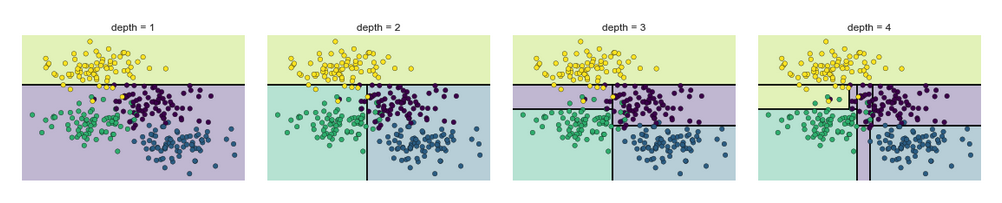
Such over-fitting turns out to be a general drawback of decision trees: it is very easy to go too deep in the tree, and thus to fit details of the particular data rather than the overall properties of the distributions they are drawn from. Another way to see this over-fitting is to look at models trained on different subsets of the data—for example, in this figure we train two different trees, each on half of the original data:
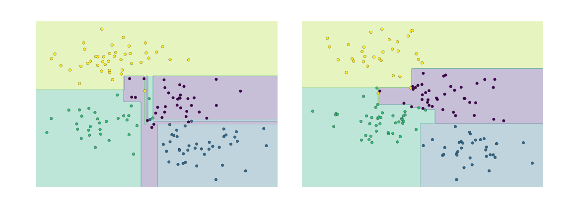
It is clear that in some places, the two trees produce consistent results (e.g., in the four corners), while in other places, the two trees give very different classifications (e.g., in the regions between any two clusters). The key observation is that the inconsistencies tend to happen where the classification is less certain, and thus by using information from both of these trees, we might come up with a better result!
Note
In signal processing a similar concept called solution stacking is employed to improve instrument resolution “after the fact.” Synthetic Arpature Radar (SAR) is a good example of solution stacking (a kind of regression tree) to improve apparent signal resolution>
Just as using information from two trees improves our results, we might expect that using information from many trees would improve our results even further. AND WHAT WOULD WE HAVE IF WE HAD MANY TREES?
YES! A FOREST! (If we had many Ents (smart trees ;) ), we could have Fangorn Forest!)

This notion—that multiple overfitting estimators can be combined to reduce the effect of this overfitting—is what underlies an ensemble method called bagging. Bagging makes use of an ensemble (a grab bag, perhaps) of parallel estimators, each of which over-fits the data, and averages the results to find a better classification. An ensemble of randomized decision trees is known as a random forest.
What is Random Forest?#
Random Forest is a versatile machine learning method capable of performing both regression and classification tasks. It also undertakes dimensional reduction methods, treats missing values, outlier values and other essential steps of data exploration, and does a fairly good job. It is a type of ensemble learning method, where a group of weak models combine to form a powerful model.
In Random Forest, we grow multiple trees. To classify a new object based on attributes, each tree gives a classification and we say the tree “votes” for that class. The forest chooses the classification having the most votes (over all the trees in the forest) and in case of regression, it takes the average of outputs by different trees.
How Random Forest algorithm works?#
Random forest is like bootstrapping algorithm with Decision tree (CART) model. Say, we have 1000 observation in the complete population with 10 variables. Random forest tries to build multiple CART models with different samples and different initial variables. For instance, it will take a random sample of 100 observation and 5 randomly chosen initial variables to build a CART model. It will repeat the process (say) 10 times and then make a final prediction on each observation. Final prediction is a function of each prediction. This final prediction can simply be the mean of each prediction. Let’s consider an imaginary example:
Out of a large population, Say, the algorithm Random forest picks up 10k observation with only one variable (for simplicity) to build each CART model. In total, we are looking at 5 CART model being built with different variables. In a real life problem, you will have more number of population sample and different combinations of input variables. The target variable is the salary bands:
Band1 : Below 40000
Band2 : 40000 - 150000
Band3 : Above 150000
Following are the outputs of the 5 different CART model:
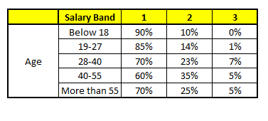
CART1 : Based on “Age” as predictor:#
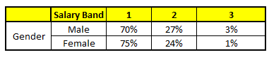
CART2 : Based on “Gender” as predictor:#
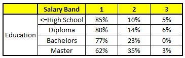
CART3 : Based on “Education” as predictor:#
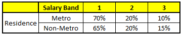
CART4 : Based on “Residence” as predictor:#
CART5 : Based on “Industry” as predictor:#
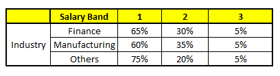
Using these 5 CART models, we need to come up with single set of probability to belong to each of the salary classes. For simplicity, we will just take a mean of probabilities in this case study. Other than simple mean, we also consider vote method to come up with the final prediction. To come up with the final prediction let’s locate the following profile in each CART model:
Age : 35 years
Gender : Male
Highest Educational Qualification : Diploma holder
Industry : Manufacturing
Residence : Metro
For each of these CART model, following is the distribution across salary bands :
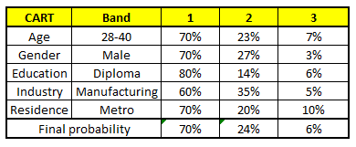
The final probability is simply the average of the probability in the same salary bands in different CART models. As you can see from this analysis, that there is 70% chance of this individual falling in class 1 (less than 40,000) and around 24% chance of the individual falling in class 2.
8.1 Iris Plants Classification by Random Forest
#
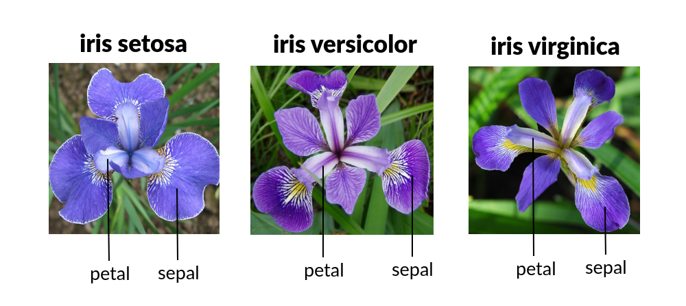
The Iris Flower Dataset involves predicting the flower species given measurements of iris flowers. The Iris Data Set contains information on sepal length, sepal width, petal length, petal width all in cm, and class of iris plants. The data set contains 3 classes of 50 instances each.
Let’s use Random Forest in Python and see if we can classifity iris plants based on the four given predictors.
Note
The Iris classification example that follows is largely sourced from:
Fisher,R.A. “The use of multiple measurements in taxonomic problems” Annual Eugenics, 7, Part II, 179-188 (1936); also in “Contributions to Mathematical Statistics” (John Wiley, NY, 1950).
Duda,R.O., & Hart,P.E. (1973) Pattern Classification and Scene Analysis. (Q327.D83) John Wiley & Sons. ISBN 0-471-22361-1. See page 218.
Dasarathy, B.V. (1980) “Nosing Around the Neighborhood: A New System Structure and Classification Rule for Recognition in Partially Exposed Environments”. IEEE Transactions on Pattern Analysis and Machine Intelligence, Vol. PAMI-2, No. 1, 67-71.
Gates, G.W. (1972) “The Reduced Nearest Neighbor Rule”. IEEE Transactions on Information Theory, May 1972, 431-433.
See also: 1988 MLC Proceedings, 54-64. Cheeseman et al’s AUTOCLASS II conceptual clustering system finds 3 classes in the data.
import numpy as np
import pandas as pd
from matplotlib import pyplot as plt
import sklearn.metrics as metrics
import seaborn as sns
%matplotlib inline
# Read the remote database directly from its url (Jupyter):
url = "https://archive.ics.uci.edu/ml/machine-learning-databases/iris/iris.data"
# Assign colum names to the dataset
names = ['sepal-length', 'sepal-width', 'petal-length', 'petal-width', 'Class']
# Read dataset to pandas dataframe
dataset = pd.read_csv(url, names=names)
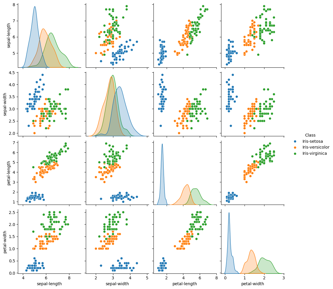
sns.pairplot(dataset, hue='Class') #A very cool plot to explore a dataset
# Notice that iris-setosa is easily identifiable by petal length and petal width,
# while the other two species are much more difficult to distinguish.
<seaborn.axisgrid.PairGrid at 0x702f741d70d0>
dataset.tail()
| sepal-length | sepal-width | petal-length | petal-width | Class | |
|---|---|---|---|---|---|
| 145 | 6.7 | 3.0 | 5.2 | 2.3 | Iris-virginica |
| 146 | 6.3 | 2.5 | 5.0 | 1.9 | Iris-virginica |
| 147 | 6.5 | 3.0 | 5.2 | 2.0 | Iris-virginica |
| 148 | 6.2 | 3.4 | 5.4 | 2.3 | Iris-virginica |
| 149 | 5.9 | 3.0 | 5.1 | 1.8 | Iris-virginica |
X = dataset.iloc[:, :-1].values
y = dataset.iloc[:, 4].values
from sklearn.model_selection import train_test_split
X_train, X_test, y_train, y_test = train_test_split(X, y, test_size=0.75)
from sklearn.ensemble import RandomForestClassifier
rf = RandomForestClassifier(n_estimators=100, oob_score=True, random_state=123456)
rf.fit(X_train, y_train)
predicted = rf.predict(X_test)
myx = [[3	,3,	1,	2.5]]
rf.predict(myx)
array(['Iris-setosa'], dtype=object)
from sklearn.metrics import classification_report, confusion_matrix, roc_auc_score

def summarize_rf_model(rf, X_train, y_train, X_test, y_test, predicted, probabilities=None):
    print("Random Forest Summary:")
    print(f"- OOB Score (if enabled): {getattr(rf, 'oob_score_', 'N/A')}")
    print(f"- Train Accuracy: {rf.score(X_train, y_train):.3f}")
    print(f"- Test Accuracy: {rf.score(X_test, y_test):.3f}")
    print(f"- Classes: {rf.classes_}")
    print(f"- Number of Features: {rf.n_features_in_}")

    print("\n Classification Report:")
    print(classification_report(y_test, predicted))

    print(" Confusion Matrix:")
    print(confusion_matrix(y_test, predicted))

    if probabilities is not None and rf.n_classes_ == 2:
        roc_auc = roc_auc_score(y_test, probabilities[:, 1])
        print(f"\n🔍 ROC AUC Score: {roc_auc:.3f}")
predicted = rf.predict(X_test)
probabilities = rf.predict_proba(X_test)
summarize_rf_model(rf, X_train, y_train, X_test, y_test, predicted, probabilities)
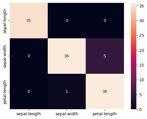
cm = pd.DataFrame(confusion_matrix(y_test, predicted), columns=names[0:3], index=names[0:3])
sns.heatmap(cm, annot=True)
Random Forest Summary:
- OOB Score (if enabled): 0.9459459459459459
- Train Accuracy: 1.000
- Test Accuracy: 0.947
- Classes: ['Iris-setosa' 'Iris-versicolor' 'Iris-virginica']
- Number of Features: 4

 Classification Report:
                 precision    recall  f1-score   support

    Iris-setosa       1.00      1.00      1.00        35
Iris-versicolor       0.97      0.88      0.92        41
 Iris-virginica       0.88      0.97      0.92        37

       accuracy                           0.95       113
      macro avg       0.95      0.95      0.95       113
   weighted avg       0.95      0.95      0.95       113

 Confusion Matrix:
[[35  0  0]
 [ 0 36  5]
 [ 0  1 36]]
<Axes: >
import matplotlib.pyplot as plt
import numpy as np
import pandas as pd

def plot_feature_importance(rf, feature_names, top_n=10):
    importances = rf.feature_importances_
    indices = np.argsort(importances)[::-1][:top_n]

    top_features = [feature_names[i] for i in indices]
    top_importances = importances[indices]

    plt.figure(figsize=(10, 6))
    plt.barh(range(len(top_importances)), top_importances[::-1], align='center')
    plt.yticks(range(len(top_importances)), top_features[::-1])
    plt.xlabel("Feature Importance")
    plt.title("Top Feature Importances from Random Forest")
    plt.tight_layout()
    plt.show()
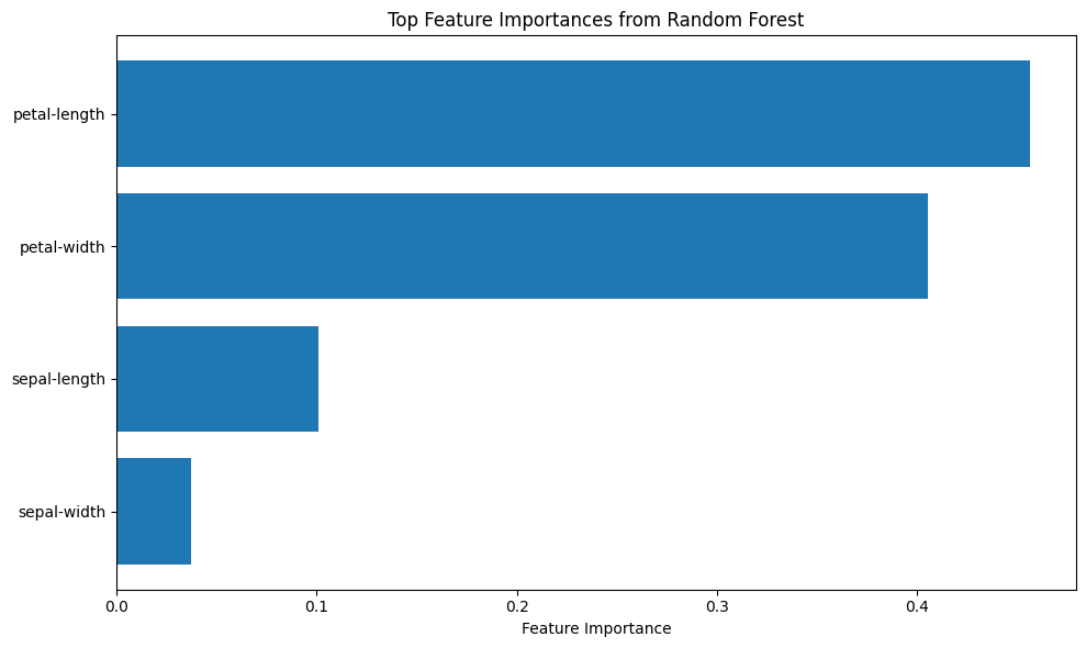
plot_feature_importance(rf, names, top_n=15)
8.1 Poison Mushroom using Random Forest#
# 8.1 OpenAI assisted code for Random Forest Method
##########################################################################################################################
##### Encoding definitions: (ordered list of categories, starting index for ordinal encoding)#############################
##########################################################################################################################
encodings = {
'poison-class': (['e', 'p'], 0),
'cap-shape': (['b','c','x','f','k','s'], 1),
'cap-surface': (['f','g','y','s'], 1),
'cap-color': (['n','b','c','g','r','p','u','e','w','y'], 1),
'bruises': (['f','t'], 1),
'odor': (['a','l','c','y','f','m','n','p','s'], 1),
'gill-attachment': (['a','d','f','n'], 1),
'gill-spacing': (['c','w','d'], 1),
'gill-size': (['b','n'], 1),
'gill-color': (['k','n','b','h','g','r','o','p','u','e','w','y'], 1),
'stalk-shape': (['e','t'], 1),
'stalk-root': (['b','c','u','e','z','r','?'], 1),
'stalk-surface-above-ring':(['f','y','k','s','?'], 1),
'stalk-surface-below-ring':(['f','y','k','s','?'], 1),
'stalk-color-above-ring': (['n','b','c','g','o','p','e','w','y'], 1),
'stalk-color-below-ring': (['n','b','c','g','o','p','e','w','y'], 1),
'veil-type': (['p','u'], 1),
'veil-color': (['n','o','w','y'], 1),
'ring-number': (['n','o','t'], 1),
'ring-type': (['c','e','f','l','n','p','s','z'], 1),
'spore-print-color': (['k','n','b','h','r','o','u','w','y','?'], 1),
'population': (['a','c','n','s','v','y','?'], 1),
'habitat': (['g','l','m','p','u','w','d'], 1)
}
##########################################################################################################################
###### Define Encoder Generator ##########################################################################################
##########################################################################################################################
def make_encoder(alphabet, offset=1, name='feature'):
def encoder(val):
if val in alphabet:
return alphabet.index(val) + offset
raise Exception(f"Encoding failed in '{name}': unknown value '{val}'")
return encoder
##########################################################################################################################
##### Apply Encodings ####################################################################################################
##########################################################################################################################
from pandas import get_dummies
def apply_encodings(df, encodings, method="ordinal"):
encoded_df = pd.DataFrame(index=df.index)
for col, (alphabet, offset) in encodings.items():
if method == "ordinal":
encoder = make_encoder(alphabet, offset=offset, name=col)
encoded_df[col] = df[col].apply(encoder)
elif method == "onehot":
df[col] = pd.Categorical(df[col], categories=alphabet, ordered=True)
dummies = get_dummies(df[col], prefix=col)
encoded_df = pd.concat([encoded_df, dummies], axis=1)
else:
raise ValueError("Unknown encoding method: use 'ordinal' or 'onehot'")
return encoded_df
##########################################################################################################################
##### Report Generator ###################################################################################################
##########################################################################################################################
def generate_encoding_markdown(encodings):
md = "# Mushroom Feature Encoding Reference\n\n"
for feature, (alphabet, offset) in encodings.items():
md += f"### {feature}\n"
md += "| Category | Encoded Value |\n"
md += "|----------|----------------|\n"
for i, symbol in enumerate(alphabet):
md += f"| `{symbol}` | `{i + offset}` |\n"
md += "\n"
return md
#########################################################################################################################
###### Step 1: Load the raw data ########################################################################################
#########################################################################################################################
###### Get the database (unchanged from original code)
import sys # Module to process commands to/from the OS using a shell-type syntax
import requests
remote_url="http://54.243.252.9/ce-5319-webroot/ce5319jb/lessons/logisticregression/agaricus-lepiota.data" # set the url
rget = requests.get(remote_url, allow_redirects=True) # get the remote resource, follow imbedded links
localfile = open('poisonmushroom.csv','wb') # open connection to a local file same name as remote
localfile.write(rget.content) # extract from the remote the contents,insert into the local file same name
localfile.close() # close connection to the local file
###### Read and load data into dataframe, set column names to the encoding keys
mymushroom = pd.read_csv('poisonmushroom.csv', header=None)
mymushroom.columns = list(encodings.keys())
#########################################################################################################################
###### Step 2: Encode ###################################################################################################
#########################################################################################################################
interim = apply_encodings(mymushroom.copy(), encodings, method="ordinal") # or "onehot"
#########################################################################################################################
###### Step 3: Export Markdown (optional) ###############################################################################
#########################################################################################################################
md_report = generate_encoding_markdown(encodings)
with open("encoding_reference.md", "w") as f:
f.write(md_report)
interim.head()
#########################################################################################################################
###### Step 4: Split Dataframe for Training, Testing ###################################################################
#########################################################################################################################
feature_cols = mymushroom.columns[1:] #split dataset in features and target variable
X = interim[feature_cols] # Features
y = interim['poison-class'] # Target variable
# split X and y into training and testing sets
from sklearn.model_selection import train_test_split
X_train,X_test,y_train,y_test=train_test_split(X,y,test_size=0.25,random_state=0)
#########################################################################################################################
###### Step 5: Load Random Forest Classifier, Fit Data Model ##########################################################
#########################################################################################################################
from sklearn.ensemble import RandomForestClassifier
rf = RandomForestClassifier(
n_estimators=100,
random_state=123456,
oob_score=True
)
rf.fit(X_train, y_train)
y_pred = rf.predict(X_test)
print("Random Forest Classifier")
print("OOB Score:", rf.oob_score_)
print("Training Accuracy:", rf.score(X_train, y_train))
print("Test Accuracy:", rf.score(X_test, y_test))
from sklearn import metrics
cnf_matrix = metrics.confusion_matrix(y_test, y_pred)
import matplotlib.pyplot as plt
import seaborn as sns
import numpy as np
import pandas as pd
class_names = [0, 1]
fig, ax = plt.subplots()
tick_marks = np.arange(len(class_names))
plt.xticks(tick_marks, class_names)
plt.yticks(tick_marks, class_names)
sns.heatmap(pd.DataFrame(cnf_matrix), annot=True, cmap="YlGnBu", fmt='g')
ax.xaxis.set_label_position("top")
plt.tight_layout()
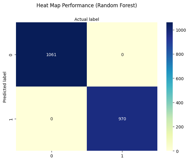
plt.title('Heat Map Performance (Random Forest)', y=1.1)
plt.ylabel('Predicted label')
plt.xlabel('Actual label');
#########################################################################################################################
###### Step 7: Classify New Mushroom ###################################################################################
#########################################################################################################################
s_new = "csgfnfwbktrssggpwoeksu" # Sample input string from a new mushroom (22 characters)
# Create encoders from the original encoding dictionary
encoders = {
col: make_encoder(alphabet, offset=offset, name=col)
for col, (alphabet, offset) in encodings.items()
}
# Get list of feature columns (excluding 'poison-class')
feature_cols = list(encodings.keys())[1:] # skip target
# Zip characters with corresponding features
try:
x_new = [encoders[col](char) for col, char in zip(feature_cols, s_new)]
except Exception as e:
print("Encoding error:", e)
x_new = None
# Predict if encoding successful
if x_new:
y_new = rf.predict(np.array(x_new).reshape(1, -1))
if y_new < 1:
print("\033[92mNew mushroom classified as EDIBLE\033[0m") # Green text
else:
print("\033[91mNew mushroom classified as POISONOUS\033[0m") # Red text
Random Forest Classifier
OOB Score: 1.0
Training Accuracy: 1.0
Test Accuracy: 1.0
New mushroom classified as EDIBLE
/opt/jupyterhub/lib/python3.10/site-packages/sklearn/utils/validation.py:2739: UserWarning: X does not have valid feature names, but RandomForestClassifier was fitted with feature names
  warnings.warn(
importances = rf.feature_importances_
sorted_idx = np.argsort(importances)[::-1]
plt.figure(figsize=(10, 6))
plt.bar(range(len(sorted_idx)), importances[sorted_idx])
plt.xticks(range(len(sorted_idx)), X.columns[sorted_idx], rotation=90)
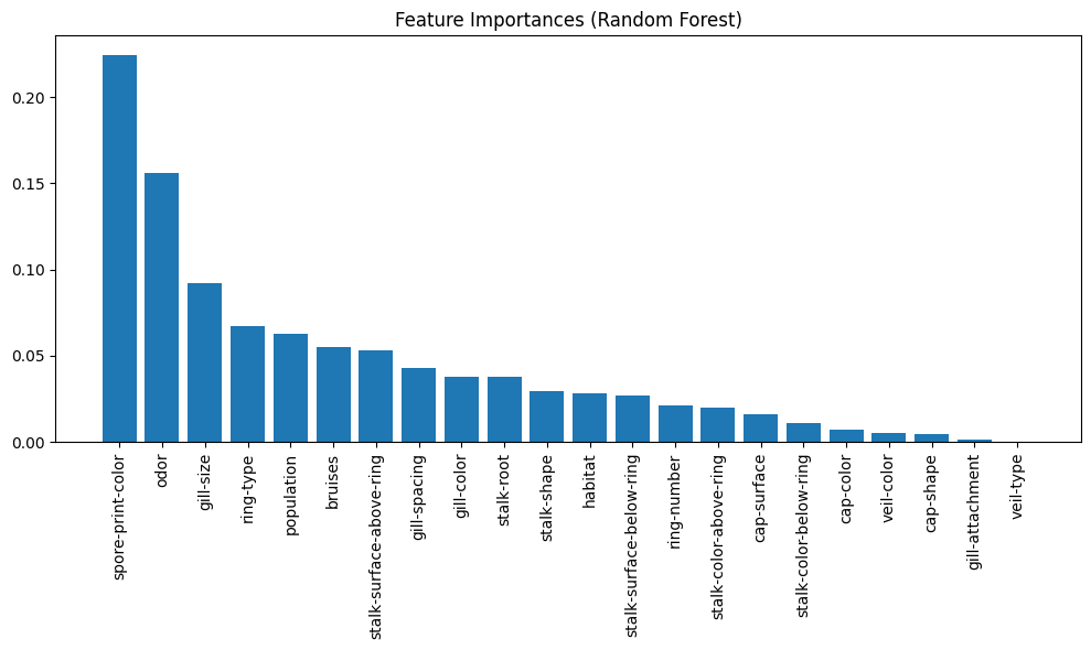
plt.title("Feature Importances (Random Forest)")
plt.tight_layout()
plt.show()
Tip
Logistic regression does not naturally produce a visually interpretable feature importance plot—its coefficients are linear weights, which can be difficult to interpret, especially when features are on arbitrary categorical scales.
However, when using models like decision trees or random forests, we can generate feature importance plots that highlight which inputs contribute most to the prediction. These plots are useful for dimensionality reduction, helping us identify and potentially eliminate low-impact features to simplify the model, reduce overfitting risk, or improve computational efficiency.
Note
There is often a trade-off between model interpretability and predictive performance.
Logistic regression offers high interpretability—its coefficients directly relate each feature to the predicted outcome under a linear model assumption. This makes it easy to explain to stakeholders or document in regulatory settings. However, it may struggle to capture complex interactions or nonlinear patterns in the data.
Random forests, on the other hand, usually deliver better predictive performance on categorical and nonlinear problems like this mushroom classification task. They model interactions and nonlinearities automatically, but their inner workings are harder to explain—a single prediction is the result of aggregated decisions across many trees, which makes direct interpretation more difficult.
When designing machine learning tools for real-world applications, it’s important to balance these two concerns depending on the audience, risk, and use case.
feature_cols[2]
'cap-color'
Model Comparison: Interpretability vs. Predictive Power#
Model |
Interpretability |
Captures Nonlinearity |
Handles Categorical Features |
Typical Use Case |
|---|---|---|---|---|
Logistic Regression |
⭐⭐⭐⭐⭐ (High) |
❌ No |
⚠️ Needs manual encoding |
Baseline classifier, regulatory reporting |
Decision Tree |
⭐⭐⭐ (Medium) |
✅ Yes |
✅ Native support |
Simple rule-based systems, visualization |
Random Forest |
⭐⭐ (Low) |
✅ Yes |
✅ Native support |
High-accuracy classification tasks |
Support Vector Machine |
⭐ (Low) |
✅ Yes (via kernels) |
⚠️ Needs preprocessing |
Small feature sets with clear boundaries |
Neural Network (MLP) |
⭐ (Very Low) |
✅✅✅ Yes (deep) |
⚠️ Needs preprocessing |
Complex or high-dimensional data patterns |
⚠️ Manual encoding often means one-hot or ordinal encoding before model input.
Note
Interpretability and accuracy are often in tension. In regulated domains or educational settings, a simpler model may be preferable even if it performs slightly worse. In critical classification tasks (like medical triage or safety systems), both high interpretability and performance may be required.
Engineering Application(s) Examples#
General Observations Regarding Random Forests#
Pros:#
this algorithm can solve both type of problems i.e. classification and regression and does a decent estimation at both fronts.
It is effective in high dimensional spaces.
One of the most essential benefits of Random forest is, the power to handle large data sets with higher dimensionality. It can handle thousands of input variables and identify most significant variables so it is considered as one of the dimensionality reduction methods. Further, the model outputs Importance of variable, which can be a very handy feature.
It has an effective method for estimating missing data and maintains accuracy when a large proportion of the data are missing.
It has methods for balancing errors in datasets where classes are imbalanced.
The capabilities of the above can be extended to unlabeled data, leading to unsupervised clustering, data views and outlier detection.
Both training and prediction are very fast, because of the simplicity of the underlying decision trees. In addition, both tasks can be straightforwardly parallelized, because the individual trees are entirely independent entities.**
The nonparametric model is extremely flexible, and can thus perform well on tasks that are under-fit by other estimators.
Cons:#
It surely does a good job at classification but not as good as for regression problem as it does not give continuous output. In case of regression, it doesn’t predict beyond the range in the training data, and that they may over-fit data sets that are particularly noisy.
Random Forest can feel like a black box approach for statistical modelers – you have very little control on what the model does. You can at best – try different parameters and random seeds!