8. Nearest Neighbor Methods#
Course Website
The K-nearest neighbors (KNN) algorithm is a type of supervised machine learning algorithms. KNN is easy to implement in its most basic form, and yet performs quite complex classification tasks. It is a lazy learning algorithm because it doesn’t have a specialized training phase. Rather, it uses all of the data for training while classifying a new data point or instance. KNN is a non-parametric learning algorithm, which means that it doesn’t assume anything about the underlying data. This is an extremely useful feature since most of the real world data doesn’t really follow any theoretical assumption.
Readings#
Chan, Jamie. Machine Learning With Python For Beginners: A Step-By-Step Guide with Hands-On Projects (Learn Coding Fast with Hands-On Project Book 7) (p. 2). Kindle Edition.
Burkov, A. (2019) “The Hundred Page Machine Learning Book” pp. 15-16
Sampaio, C. (2022) “K-Nearest Neighbors Algorithm in Python and Scikit-Learn”
Brownlee, J. (2019) “Develop k-Nearest Neighbors in Python From Scratch”
Brownlee, J. (2020) “4 Distance Measures for Machine Learning”
tavishaggarwal1993 (2022) “k-nearest neighbor algorithm in Python” Author’s name is an avatar
Videos#
Attribution
This section on KNN Classification is largely copied from Theodore G. Cleveland, Farhang Forghanparast (2021), Computational Thinking and Data Science: Instructor’s Notes for ENGR 1330 at TTU, with contributions by: Dinesh Sundaravadivelu Devarajan, Turgut Batuhan Baturalp (Batu), Tanja Karp, Long Nguyen, and Mona Rizvi. Whitacre College of Engineering, DOI (pending) .
A description from https://en.wikipedia.org/wiki/K-nearest_neighbors_algorithm is:
In statistics, the k-nearest neighbors algorithm (k-NN) is a non-parametric classification method first developed by Evelyn Fix and Joseph Hodges in 1951, and later expanded by Thomas Cover. It is used for classification and regression. In both cases, the input consists of the k closest training examples in a data set. The output depends on whether k-NN is used for classification or regression:
In k-NN classification, the output is a class membership. An object is classified by a plurality vote of its neighbors, with the object being assigned to the class most common among its k nearest neighbors (k is a positive integer, typically small). If k = 1, then the object is simply assigned to the class of that single nearest neighbor.
In k-NN regression, the output is the property value for the object. This value is the average of the values of k nearest neighbors.
k-NN is a type of classification where the function is only approximated locally and all computation is deferred until function evaluation. Since this algorithm relies on distance for classification, if the features represent different physical units or come in vastly different scales then normalizing the training data can improve its accuracy dramatically.
Both for classification and regression, a useful technique can be to assign weights to the contributions of the neighbors, so that the nearer neighbors contribute more to the average than the more distant ones. For example, a common weighting scheme consists in giving each neighbor a weight of 1/d, where d is the distance to the neighbor.
The neighbors are taken from a set of objects for which the class (for k-NN classification) or the object property value (for k-NN regression) is known. This can be thought of as the training set for the algorithm, though no explicit training step is required.
A peculiarity of the k-NN algorithm is that it is sensitive to the local structure of the data. …
KNN Background#
The First Law of Geography, according to Waldo Tobler, is “everything is related to everything else, but near things are more related than distant things.” The intuition behind the KNN algorithm is one of the simplest of all the supervised machine learning algorithms:
It calculates the distance of a new data point to all other training data points.
The distance can be of any type e.g Euclidean or Manhattan etc.
It then selects the K-nearest data points, where K can be any integer.
Used as a classifier; it assigns the data point to the class to which the majority of the K data points belong.
Used as a predictor; it assigns to the data point a mean prediction value based on the associated values of the K data points.
KNN as a prediction engine is demonstrated in the SolidsInRivers tool. The underlying code—excluding the web interface and server configurations—is detailed later in the KNN Regression subsection.
Concept of Distance in N-Dimensional Space#
The concept of distance is vital to search engines; hence distance measures play an important role in machine learning. Three common used distance measures in machine learning are as follows:

Euclidean Distance: Calculates the distance between two real-valued vectors. Although there are other possible choices, most instance-based learners use Euclidean distance.
Manhattan Distance: Also called the Taxicab distance or the City Block distance, calculates the distance between two real-valued vectors. It is perhaps more useful to vectors that describe objects on a uniform grid, like a chessboard or city blocks. The taxicab name for the measure refers to the intuition for what the measure calculates: the shortest path that a taxicab would take between city blocks (coordinates on the grid).
Minkowski Distance: Calculates the distance between two real-valued vectors. It is a generalization of the Euclidean and Manhattan distance measures and adds a parameter, called the “order” or “p“, that allows different distance measures to be calculated. When p is set to 1, the calculation is the same as the Manhattan distance. When p is set to 2, it is the same as the Euclidean distance.
The SolidsInRivers estimation tool, allows the user to specify the exponent in a Minkowski distance measure, and select the neighbor count (K). Then it searches the database for the K nearest neighbors, and returns an estimate that is the arithmetic mean of these K values.
Data Normalization#
In KNN application the scale of predictors influences results; when the variables in the database are not expressed in the same magnitude, range, and scale. If values of one predictor are several orders of magnitude larger in the database than another predictor, the two are not directly comparable when computing a distance for the search algorithm. In such a case, one way to facilitate direct interpretation for comparing composite indices of the original data having different magnitudes and unit systems is to use normalization. Normalization serves the purpose of bringing the indicators into the same unit scale or unit base and makes distance computations appropriate. Normalizing data is done using various standardization techniques to assign a value to each variable so that they may be directly compared without unintentional bias due to differences in unit scale.
Z-score Standardization#
Z-score standardization is a commonly used normalization method that converts all indicators to a common scale with an average of zero and standard deviation of one. This transformation is the same as computing a standard-normal score for each data value.
\(Z = \frac{x-\mu}{\sigma}\)
where:
\(x\) = Data point value
\(\mu\) = Mean
\(\sigma\) = Standard Deviation
The average of zero avoids the introduction of aggregation distortions stemming from differences in indicators’ means. The scaling factor is the standard deviation of the indicator across the various predictors being ranked. Thus, an indicator with extreme values will have intrinsically a greater effect on the composite indicator. The raw score on each data entry is converted to a Z-score, then distances are calculated using the Z-scores for each variable rather than the raw value. Upon completion of the distance calculations and selection of the nearest neighbors, the results are transformed back into the original values for subsequent presentation. Unit-Interval
[0,1] Standardization#
An alternate approach for standardization is to use a mapping of each variable in the database to a [0,1] scale and linearly weight within the scale. This standardization has the same goal as Z-score, which is to prevent one variable from overwhelming the distance computations because of its relative magnitude. The unit interval [0,1] standardization technique differs from the Z-score in that the variability is governed by the minimum and maximum value for each variable, and hence extrapolation is not feasible. Because extrapolation is likely necessary until new records are added to any database, this standardization method is often useless.
8.1 KNN Classification#
Let’s see this algorithm in action with the help of a simple example. Suppose you have a dataset with two variables, which when plotted, looks like the one in the following figure.
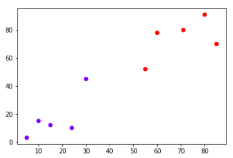
Your task is to classify a new data point with ‘X’ into “Blue” class or “Red” class. The coordinate values of the data point are x=45 and y=50. Suppose the value of K is 3. The KNN algorithm starts by calculating the distance of point X from all the points. It then finds the 3 nearest points with least distance to point X. This is shown in the figure below. The three nearest points have been encircled.
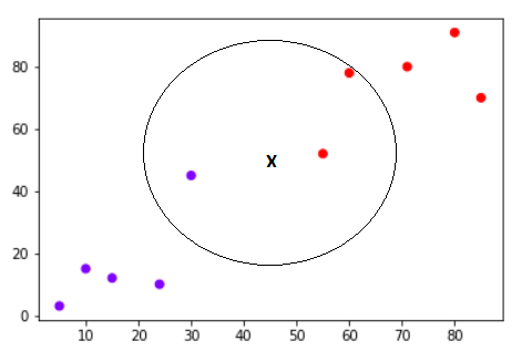
The final step of the KNN algorithm is to assign new point to the class to which majority of the three nearest points belong. From the figure above we can see that the two of the three nearest points belong to the class “Red” while one belongs to the class “Blue”. Therefore the new data point will be classified as “Red”.

Why KNN?#

It is extremely easy to implement
It is lazy learning algorithm and therefore requires no training prior to making real time predictions. This makes the KNN algorithm much faster than other algorithms that require training e.g SVM, linear regression, etc.
Because the algorithm requires no training before making predictions, new data can be added seamlessly.
There are only two parameters required to implement KNN i.e. the value of K and the distance function (e.g. Euclidean or Manhattan etc.)
Classic Example: Iris Plants Classification
#

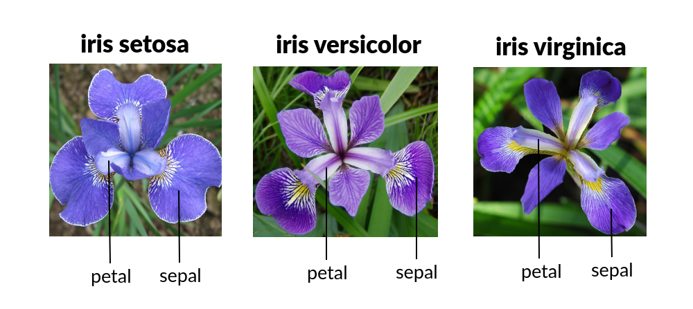
This is a well known problem and database to be found in the pattern recognition literature. Fisher’s paper is a classic in the field and is referenced frequently to this day. The Iris Flower Dataset involves predicting the flower species given measurements of iris flowers.
The Iris Data Set contains information on sepal length, sepal width, petal length, petal width all in cm, and class of iris plants. The data set contains 3 classes of 50 instances each, where each class refers to a type of iris plant. Hence, it is a multiclass classification problem and the number of observations for each class is balanced.
Let’s use a KNN model in Python and see if we can classifity iris plants based on the four given predictors.
Note
The Iris classification example that follows is largely sourced from:
Fisher,R.A. “The use of multiple measurements in taxonomic problems” Annual Eugenics, 7, Part II, 179-188 (1936); also in “Contributions to Mathematical Statistics” (John Wiley, NY, 1950).
Duda,R.O., & Hart,P.E. (1973) Pattern Classification and Scene Analysis. (Q327.D83) John Wiley & Sons. ISBN 0-471-22361-1. See page 218.
Dasarathy, B.V. (1980) “Nosing Around the Neighborhood: A New System Structure and Classification Rule for Recognition in Partially Exposed Environments”. IEEE Transactions on Pattern Analysis and Machine Intelligence, Vol. PAMI-2, No. 1, 67-71.
Gates, G.W. (1972) “The Reduced Nearest Neighbor Rule”. IEEE Transactions on Information Theory, May 1972, 431-433.
See also: 1988 MLC Proceedings, 54-64. Cheeseman et al’s AUTOCLASS II conceptual clustering system finds 3 classes in the data.
Load some libraries:
import numpy as np
import pandas as pd
from matplotlib import pyplot as plt
import sklearn.metrics as metrics
import seaborn as sns
%matplotlib inline
Read the dataset and explore it using tools such as descriptive statistics:
# Read the remote directly from its url (Jupyter):
url = "https://archive.ics.uci.edu/ml/machine-learning-databases/iris/iris.data"
# Assign colum names to the dataset
names = ['sepal-length', 'sepal-width', 'petal-length', 'petal-width', 'Class']
# Read dataset to pandas dataframe
dataset = pd.read_csv(url, names=names)
dataset.tail()
| sepal-length | sepal-width | petal-length | petal-width | Class | |
|---|---|---|---|---|---|
| 145 | 6.7 | 3.0 | 5.2 | 2.3 | Iris-virginica |
| 146 | 6.3 | 2.5 | 5.0 | 1.9 | Iris-virginica |
| 147 | 6.5 | 3.0 | 5.2 | 2.0 | Iris-virginica |
| 148 | 6.2 | 3.4 | 5.4 | 2.3 | Iris-virginica |
| 149 | 5.9 | 3.0 | 5.1 | 1.8 | Iris-virginica |
dataset.describe()
| sepal-length | sepal-width | petal-length | petal-width | |
|---|---|---|---|---|
| count | 150.000000 | 150.000000 | 150.000000 | 150.000000 |
| mean | 5.843333 | 3.054000 | 3.758667 | 1.198667 |
| std | 0.828066 | 0.433594 | 1.764420 | 0.763161 |
| min | 4.300000 | 2.000000 | 1.000000 | 0.100000 |
| 25% | 5.100000 | 2.800000 | 1.600000 | 0.300000 |
| 50% | 5.800000 | 3.000000 | 4.350000 | 1.300000 |
| 75% | 6.400000 | 3.300000 | 5.100000 | 1.800000 |
| max | 7.900000 | 4.400000 | 6.900000 | 2.500000 |
Split the predictors and target - similar to what we did for logisitc regression:
X = dataset.iloc[:, :-1].values
y = dataset.iloc[:, 4].values
Then, the dataset should be split into training and testing. This way our algorithm is tested on un-seen data, as it would be in a real-world application. Let’s go with a 80/20 split:
from sklearn.model_selection import train_test_split
X_train, X_test, y_train, y_test = train_test_split(X, y, test_size=0.2)

#This means that out of total 150 records:
#the training set will contain 120 records &
#the test set contains 30 of those records.
It is extremely straight forward to train the KNN algorithm and make predictions with it, especially when using Scikit-Learn. The first step is to import the “KNeighborsClassifier” class from the “sklearn.neighbors” library. In the second line, this class is initialized with one parameter, i.e. “n_neigbours”. This is basically the value for the K. There is no ideal value for K and it is selected after testing and evaluation, however to start out, 5 seems to be the most commonly used value for KNN algorithm.
from sklearn.neighbors import KNeighborsClassifier
classifier = KNeighborsClassifier(n_neighbors=3)
classifier.fit(X_train, y_train);
The final step is to make predictions on our test data. To do so, execute the following script:
y_pred = classifier.predict(X_test)
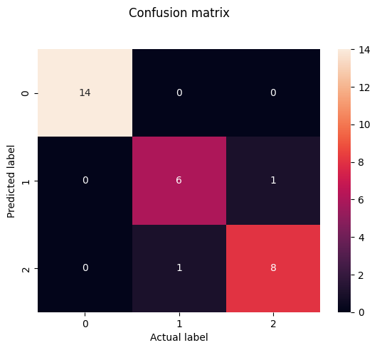
As it’s time to evaluate our model, we will go to our rather new friends, confusion matrix, precision, recall and f1 score as the most commonly used discrete GOF metrics.
from sklearn.metrics import classification_report, confusion_matrix
print(confusion_matrix(y_test, y_pred))
print(classification_report(y_test, y_pred))
[[14  0  0]
 [ 0  6  1]
 [ 0  1  8]]
                 precision    recall  f1-score   support

    Iris-setosa       1.00      1.00      1.00        14
Iris-versicolor       0.86      0.86      0.86         7
 Iris-virginica       0.89      0.89      0.89         9

       accuracy                           0.93        30
      macro avg       0.92      0.92      0.92        30
   weighted avg       0.93      0.93      0.93        30
cm = pd.DataFrame(confusion_matrix(y_test, y_pred))
sns.heatmap(cm, annot=True)
plt.title('Confusion matrix', y=1.1)
plt.ylabel('Predicted label')
plt.xlabel('Actual label')
Text(0.5, 23.52222222222222, 'Actual label')
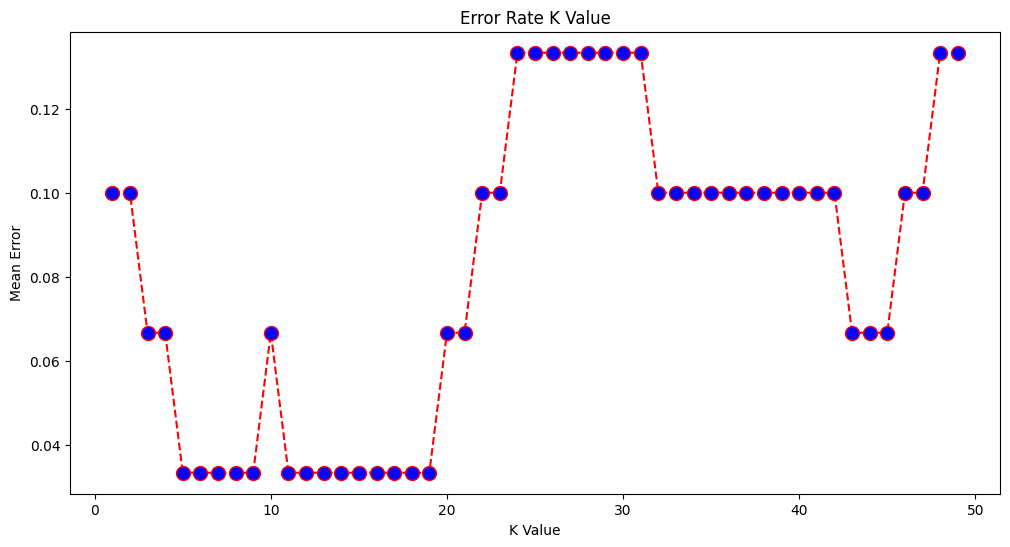
What if we had used a different value for K? What is the best value for K?
One way to help you find the best value of K is to plot the graph of K value and the corresponding error rate for the dataset. In this section, we will plot the mean error for the predicted values of test set for all the K values between 1 and 50. To do so, let’s first calculate the mean of error for all the predicted values where K ranges from 1 and 50:
error = []

# Calculating error for K values between 1 and 50
# In each iteration the mean error for predicted values of test set is calculated and
# the result is appended to the error list.
for i in range(1, 50):
    knn = KNeighborsClassifier(n_neighbors=i)
    knn.fit(X_train, y_train)
    pred_i = knn.predict(X_test)
    error.append(np.mean(pred_i != y_test))
The next step is to plot the error values against K values:
plt.figure(figsize=(12, 6))
plt.plot(range(1, 50), error, color='red', linestyle='dashed', marker='o',
         markerfacecolor='blue', markersize=10)
plt.title('Error Rate K Value')
plt.xlabel('K Value')
plt.ylabel('Mean Error')
Text(0, 0.5, 'Mean Error')
Final remarks …#
KNN is a simple yet powerful classification algorithm.
It requires no training for making predictions, which is typically one of the most difficult parts of a machine learning algorithm.
The KNN algorithm have been widely used to find document similarity and pattern recognition.
Here we presented it as a classifier, however if the output needs to be a predictor we can use “regression” type prediction using the KNN values to parameterize a data model.
We will leave the task of making classifications of new inputs for a lab exercise.
From Plants to Engineering: KNN Beyond Classification#
Classification in engineering is just as critical as in botany or biology. In the plant world, you might use physical characteristics like leaf shape or petal count to identify a species. In engineering, we might instead be classifying material types, land use categories, or soil textures based on measurable features.
But K-Nearest Neighbors (KNN) isn’t limited to classification problems. It’s just as useful for regression, where the goal is to predict a continuous value rather than assign a label.
Let’s use our pickone dataset to explore this concept in an engineering context.
8.2 KNN Regression: Same Idea, Different Target#
In KNN regression, the logic is familiar:
For a new data point (a sample with known features but unknown outcome),
Identify its k nearest neighbors in the feature space,
Then take the average of their known values (usually the mean, but sometimes a weighted average is used),
And assign that average as the prediction.
So rather than voting on a label (as in classification), we’re computing a representative numerical value.
This works particularly well in engineering applications where you have sparse or irregular data, and you want a simple but effective way to estimate an unknown based on “what’s nearby.”
When Does It Work Well?#
KNN regression is most useful when:
The data has local structure (i.e., similar inputs yield similar outputs),
You have a reasonable number of features (too many = “curse of dimensionality”),
The number of examples is small to moderate (KNN can be computationally expensive for large datasets unless optimized),
The prediction surface is nonlinear, and a simple regression might not capture it.
A Few Examples Where Engineers Might Use KNN Regression:
Estimating sediment concentration in a river based on recent rainfall, flow rate, and upstream land use.
Predicting concrete strength based on its mix composition.
Estimating pipe break likelihood based on age, material, and pressure history.
Interpolating missing sensor readings in environmental or hydrologic monitoring.
We’ll Walk Through an example based on a moderate sized database that reports solids flux in rivers based of various hydraulic and soil properties:
A homebrew example adapted from a script originally written in R,
A Python implementation using scikit-learn, showing how to make a prediction and examine nearby data points,
A visualization to help interpret what KNN regression is doing under the hood.
Attribution
The homebrew component of this subsection is derived largely from Neale, C. M. (2018). Development and Delivery of Server-Side Water Resources Models Using Web-Based Interfaces. The refactoring from the original R Script to Python was guided by this book’s author with assistance from OpenAI tools.
8.1.1 KNN Solids in Rivers (Homebrew)#
import pandas as pd
import numpy as np
import matplotlib.pyplot as plt
import seaborn as sns
import sys # Module to process commands to/from the OS using a shell-type syntax
import requests
# --- Step 1: Download database and load into a dataframe ---
filename = "solids_in_rivers.csv"
remote_url="http://54.243.252.9/ce-5319-webroot/MLBE4CE/chapters/08-nearestneighbors/solids_in_rivers.csv" # set the url
rget = requests.get(remote_url, allow_redirects=True) # get the remote resource, follow imbedded links
localfile = open(filename,'wb') # open connection to a local file same name as remote
localfile.write(rget.content) # extract from the remote the contents,insert into the local file same name
localfile.close() # close connection to the local file
df = pd.read_csv(filename) #load the dataframe
# --- Step 2: Read Input File (6 lines) ---
with open("input.dat", "r") as f:
lines = [float(line.strip()) for line in f.readlines()]
mySlope, myD50, myQ, myU, nxp, near = lines
print("Slope , D50 , Q , U , nxp , near")
print(lines)
near = int(near)
nxp = float(nxp)
# --- Step 3: Compute z-scores for DB ---
feature_names = ["S_m_m", "D50_m", "Q_m3_s", "U_m_s"]
features_z = {}
for feat in feature_names:
mu = df[feat].mean(skipna=True)
sigma = df[feat].std(skipna=True)
features_z[feat] = (df[feat] - mu) / sigma
# --- Step 4: Compute z-scores for inputs ---
myZ = {
"S_m_m": (mySlope - df["S_m_m"].mean()) / df["S_m_m"].std(),
"D50_m": (myD50 - df["D50_m"].mean()) / df["D50_m"].std(),
"Q_m3_s": (myQ - df["Q_m3_s"].mean()) / df["Q_m3_s"].std(),
"U_m_s": (myU - df["U_m_s"].mean()) / df["U_m_s"].std()
}
# --- Step 5: Compute distances ---
zdist = ((features_z["S_m_m"] - myZ["S_m_m"])**nxp +
(features_z["D50_m"] - myZ["D50_m"])**nxp +
(features_z["Q_m3_s"] - myZ["Q_m3_s"])**nxp +
(features_z["U_m_s"] - myZ["U_m_s"])**nxp) ** (1.0 / nxp)
print("Rows Remaining : ",len(zdist))
# --- Step 6: Sort and estimate ---
df["distance"] = zdist
#df_sorted = df.sort_values(by=["distance", "qb_kg_m_s"])
df_sorted = df.sort_values(by=["distance", "C_ppht"])
#nearest_qb = df_sorted["qb_kg_m_s"].iloc[:near]
nearest_qb = df_sorted["C_ppht"].iloc[:near]
estimate = nearest_qb.mean()
print(f"Estimated qb_kg_m_s: {estimate:.5f}")
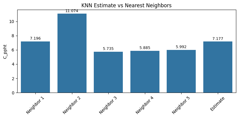
# --- Step 7: Bar Chart of 5 Nearest Neighbors + Estimate ---
bar_vals = list(nearest_qb.iloc[:5].values) + [estimate]
bar_labels = [f"Neighbor {i+1}" for i in range(min(5, near))] + ["Estimate"]
plt.figure(figsize=(8, 4))
ax = sns.barplot(x=bar_labels, y=bar_vals)
plt.ylabel("C_ppht")
plt.title("KNN Estimate vs Nearest Neighbors")
# Add value labels
for i, val in enumerate(bar_vals):
ax.text(i, val + 0.01 * max(bar_vals), f"{val:.3f}", ha='center', va='bottom', fontsize=9)
plt.xticks(rotation=45)
plt.tight_layout()
plt.show()
Slope , D50 , Q , U , nxp , near
[0.0007, 0.0013, 18.9, 1.29, 2.0, 5.0]
Rows Remaining :  12401
Estimated qb_kg_m_s: 7.17661
8.1.2 KNN Solids in Rivers#
Modernized approach using sklearn tools.
Warning
The script below is a work-in-progress using sklearn tools. The difference(s) in outcome are attributed to the “cleaning” step; the homebrew script simply skips missing features
# Load needed libaries
import pandas as pd
import numpy as np
from matplotlib import pyplot as plt
import sklearn.metrics as metrics
import seaborn as sns
%matplotlib inline
import sys # Module to process commands to/from the OS using a shell-type syntax
import requests
# --- Step 1: Download database and load into a dataframe ---
filename = "solids_in_rivers.csv"
remote_url="http://54.243.252.9/ce-5319-webroot/MLBE4CE/chapters/08-nearestneighbors/solids_in_rivers.csv" # set the url
rget = requests.get(remote_url, allow_redirects=True) # get the remote resource, follow imbedded links
localfile = open(filename,'wb') # open connection to a local file same name as remote
localfile.write(rget.content) # extract from the remote the contents,insert into the local file same name
localfile.close() # close connection to the local file
# Load dataset
df = pd.read_csv(filename) #load the dataframe
column_names = df.columns.tolist()
indices = list(range(3, 10)) + [11] + list(range(15, 17))
#indices =[3,5,9,11] # SIR WebApplication Reduced Feature Set
feature_set = [column_names[i] for i in indices]
print(feature_set)
#print(df.head())
# build target set (1 of 2)
indices = list(range(17,18))
target_set_1 = [column_names[i] for i in indices]
print(target_set_1)
# build target set (2 of 2)
indices = list(range(18,19))
target_set_2 = [column_names[i] for i in indices]
print(target_set_2)
# Build design matrix and target vectors
X = df[feature_set] # Build X design matrix
y_one = df[target_set_1]
y_two = df[target_set_2]
# Concatenate into a single DataFrame to drop rows with NaNs in any relevant part
combined = pd.concat([X, y_one, y_two], axis=1)
combined = combined.dropna()
# Re-split into X, y_one, y_two
X_clean = combined[feature_set]
y_one_clean = combined[target_set_1]
y_two_clean = combined[target_set_2]
# split sets
from sklearn.model_selection import train_test_split
X_train, X_test, y_train, y_test = train_test_split(X_clean, y_one_clean, test_size=0.1) #Split dataframe for testing
# instantiate the neighbors class
#from sklearn.neighbors import KNeighborsRegressor
#regressor = KNeighborsRegressor(n_neighbors=5,p=2)
#regressor = KNeighborsRegressor(n_neighbors=5, weights='distance', algorithm='brute', leaf_size=30, p=2, metric='minkowski', metric_params=None, n_jobs=None)
#regressor.fit(X_clean, y_one_clean)
from sklearn.preprocessing import StandardScaler
from sklearn.neighbors import KNeighborsRegressor
from sklearn.pipeline import make_pipeline
# Create a pipeline that first standardizes, then fits the regressor
regressor = make_pipeline(
StandardScaler(), # this applies Z-score transformation: (x - mean) / std
KNeighborsRegressor(n_neighbors=5, weights='distance', algorithm='brute', p=2)
)
# Fit the pipeline to the training data
regressor.fit(X_clean, y_one_clean)
# When you predict, the pipeline will apply the same transformation to the input
y_pred = regressor.predict(X_test)
print("Remaining Rows : ",len(y_one_clean))
# Predict on test set
y_pred = regressor.predict(X_test)
from sklearn.metrics import mean_squared_error, r2_score
mse = mean_squared_error(y_test, y_pred)
r2 = r2_score(y_test, y_pred)
print(f"Mean Squared Error: {mse:.3f}")
print(f"R² Score: {r2:.3f}")
# --- Define an arbitrary input vector (must match feature_set structure) ---
# Example: A vector with same order and type as your training features
# Replace with real values or user input as needed
# Wrap input in a DataFrame with correct column names
# === Prompt for user input with default fallback ===
console_prompt = False # Set to True for live server demo, otherwise leave False or Sphinx build fails
default_input = [18.9,1.29452,1.09,14.6,1.19,1.02,0.0007,0.0013,2650,999]
#default_input = [18.9,1.295,0.0007,0.0013]
values = default_input
if console_prompt:
user_input = input(f"\nEnter {len(default_input)} feature values separated by commas\n[Press Enter to use default]: ")
if user_input.strip():
try:
values = [float(x.strip()) for x in user_input.split(",")]
if len(values) != len(default_input):
raise ValueError("Incorrect number of features")
except Exception as e:
print(f"Invalid input. Using default. Reason: {e}")
values = default_input
else:
values = default_input
new_input_df = pd.DataFrame([values], columns=feature_set)
print(new_input_df.head())
# === Prediction and neighbor extraction ===
y_est = float(regressor.predict(new_input_df).item())
print(f"\nEstimated target for input: {y_est:.3f}")
#distances, indices = regressor.kneighbors(new_input_df, n_neighbors=5, return_distance=True)
#neighbor_features = X_clean.iloc[indices[0]]
#neighbor_targets = y_one_clean.iloc[indices[0]]
# Step 1: Extract the scaler and regressor
scaler = regressor.named_steps['standardscaler']
knn = regressor.named_steps['kneighborsregressor']
# Step 2: Transform the input using the scaler
X_transformed = scaler.transform(new_input_df)
# Step 3: Use kneighbors on the transformed input
distances, indices = knn.kneighbors(X_transformed, n_neighbors=5, return_distance=True)
# Step 4: Use the original (unscaled) data for reporting
neighbor_features = X_clean.iloc[indices[0]]
neighbor_targets = y_one_clean.iloc[indices[0]]
# === Print neighbor data ===
print("\n5 Nearest Neighbors:")
for i in range(5):
neighbor_target = float(neighbor_targets.iloc[i, 0])
print(f"Neighbor {i+1}:")
print(f" Distance: {distances[0][i]:.3f}")
print(f" Target: {neighbor_target:.3f}")
print(f" Features: {neighbor_features.iloc[i].values}\n")
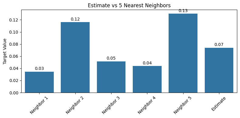
# === Plot bar chart with labels ===
labels = [f'Neighbor {i+1}' for i in range(5)] + ['Estimate']
values = list(neighbor_targets.iloc[:, 0].values) + [y_est]
plt.figure(figsize=(8, 4))
ax = sns.barplot(x=labels, y=values)
plt.ylabel("Target Value")
plt.title("Estimate vs 5 Nearest Neighbors")
# Add text labels on bars
for i, val in enumerate(values):
ax.text(i, val + 0.01 * max(values), f"{val:.2f}", ha='center', va='bottom', fontsize=10)
plt.xticks(rotation=45)
plt.tight_layout()
plt.show()
['Q_m3_s', 'q_m2_s', 'U_m_s', 'W_m', 'H_m', 'R_m', 'S_m_m', 'D50_m', 'Rhos_kg_m3', 'Rho_kg_m3']
['qb_kg_m_s']
['C_ppht']
Remaining Rows :  9260
Mean Squared Error: 0.000
R² Score: 1.000
   Q_m3_s   q_m2_s  U_m_s   W_m   H_m   R_m   S_m_m   D50_m  Rhos_kg_m3  \
0    18.9  1.29452   1.09  14.6  1.19  1.02  0.0007  0.0013        2650

   Rho_kg_m3
0        999
Estimated target for input: 0.074

5 Nearest Neighbors:
Neighbor 1:
  Distance: 0.048
  Target: 0.035
  Features: [1.89000e+01 1.29452e+00 1.09000e+00 1.46000e+01 1.19000e+00 1.02000e+00
 7.00000e-04 1.30000e-03 2.65000e+03 9.99728e+02]

Neighbor 2:
  Distance: 0.048
  Target: 0.116
  Features: [1.89000e+01 1.29452e+00 1.09000e+00 1.46000e+01 1.19000e+00 1.02000e+00
 7.00000e-04 1.30000e-03 2.65000e+03 9.99728e+02]

Neighbor 3:
  Distance: 0.052
  Target: 0.051
  Features: [1.88000e+01 1.28767e+00 1.08000e+00 1.46000e+01 1.18000e+00 1.02000e+00
 7.00000e-04 1.30000e-03 2.65000e+03 9.99728e+02]

Neighbor 4:
  Distance: 0.052
  Target: 0.044
  Features: [1.88000e+01 1.28767e+00 1.08000e+00 1.46000e+01 1.18000e+00 1.02000e+00
 7.00000e-04 1.30000e-03 2.65000e+03 9.99728e+02]

Neighbor 5:
  Distance: 0.059
  Target: 0.130
  Features: [1.96000e+01 1.34247e+00 1.10000e+00 1.46000e+01 1.22000e+00 1.04000e+00
 7.00000e-04 1.30000e-03 2.65000e+03 9.99728e+02]
Feature Importance in KNN Regression (KNeighborsRegressor)#
Unfortunately, KNeighborsRegressor does not provide feature importance directly — unlike tree-based models (like Random Forest or Gradient Boosting) which can compute importance from splits.
But common approaches to explore importance (feature engineering) are:
Permutation Importance (model-agnostic); This measures how much the prediction error increases when a feature’s values are randomly shuffled. An illustration follows below
Recursive Feature Elimination (RFE); A less common approach for KNN, but you can pair it with a wrapper model like Ridge or RandomForest to suggest a reduced feature set — or just use permutation scores above.Below is the examination for our example.
# Feature Permutation Importance examination
from sklearn.inspection import permutation_importance

result = permutation_importance(regressor, X_test, y_test, n_repeats=10, random_state=42)

# Display ranked importances
importances = result.importances_mean
sorted_idx = np.argsort(importances)[::-1]

for i in sorted_idx:
    print(f"{X_test.columns[i]}: {importances[i]:.4f}")
S_m_m: 0.9652
U_m_s: 0.3414
Rho_kg_m3: 0.1067
D50_m: 0.0764
H_m: 0.0456
R_m: 0.0414
q_m2_s: 0.0390
W_m: 0.0336
Rhos_kg_m3: 0.0297
Q_m3_s: 0.0120
The value fromresult.importances_mean gives the average change in model performance (e.g., decrease in R²) when each feature is randomly shuffled.
Meaning(s):
Higher values → more important: shuffling that feature hurts the model more.
Zero or near-zero values → model is not sensitive to that feature.
Negative values → shuffling that feature actually improves the model slightly, which suggests:
It adds noise
It’s collinear with other features
It’s irrelevant Practical Use:
Rank features by importance
Keep the top 5–6
Consider dropping features with small or negative importance
For the solid in rivers, hers is an interpretation of the output (ranked by importance):
Feature |
Importance |
Interpretation |
|---|---|---|
Rhos_kg_m3 |
0.0019 |
Most important — model relies most on sediment density |
U_m_s |
0.0018 |
Very important — velocity is a strong driver of sediment flux |
W_m |
0.0009 |
Important — probably related to wetted width or energy dissipation |
Rho_kg_m3 |
0.0006 |
Moderate — water density; not as strong as sediment density |
Q_m3_s |
0.0004 |
Minor — total flow matters, but not the dominant factor here |
H_m |
0.0002 |
Weak — flow depth has some signal but not crucial |
S_m_m |
0.0001 |
Very weak — slope has marginal influence on flux prediction in this data context |
R_m |
0.0001 |
Very weak — hydraulic radius is possibly redundant with Q and W |
q_m2_s |
0.0001 |
Very weak — unit discharge might be collinear with U or Q |
D50_m |
~0.0000 |
Not used — shuffling this doesn’t degrade model performance |
Interpretation Summary:
The data model depends mostly on:
Rhos_kg_m3 (sediment density),
U_m_s (velocity),
and to a lesser extent, W_m (channel width).
Features like D50_m (median grain size), S_m_m (slope), and q_m2_s (unit discharge) are not contributing meaningfully — possibly due to:
low variance in training data, (no sensitivity)
redundancy with other features, (colinearity - one feature is projected (dot product -> 1.0) onto another.
or poor alignment with the target (qb_kg_m_s) (the feature is fundamentally unrellated to the target).
Exercises#
# Autobuild the exercise set for this section.
import subprocess

try:
    subprocess.run(["pdflatex", "ce5319-es8-2025-2.tex"],
                   stdout=subprocess.DEVNULL, stderr=subprocess.DEVNULL, check=True)
except subprocess.CalledProcessError:
    print("Build failed. Check your LaTeX source file.")