Enumeration Methods: Grid Search#
Grid search methods are simple to conceptualize and can provide useful starting values for more elaborate tools. A substance manufacturing example below uses a simplistic grid search method that implicitly searched integer space only, here another example will use sequential searches - a first to get close to a region where good solutions exist, and a second refinement search.
Grid Search is a brute-force method for global optimization. It discretizes the search space and evaluates the objective function at every point in the grid. It’s easy to implement and guarantees that the best solution in the discretized domain is found — but at the cost of high computational expense, especially in multiple dimensions or tight step sizes.
When to Use Grid Search:#
When the problem has a small number of variables (low dimensionality).
When you want a quick first pass to identify promising regions for more refined search.
When derivative information is unavailable or unreliable.
Steps:#
Define bounds for each variable.
Choose step sizes (resolution).
Loop over combinations of variable values.
Compute the objective and constraints.
Keep the best feasible solution found.
Note
Typically one implements a coarse-to-fine grid search, where a broad sweep identifies regions of interest, and then local refinement improves solution quality.
Example: Pharmaceuticals for Fun and Profit#
Suppose you are manufacturing two substances in your dorm room, \(\textbf{A}\) and \(\textbf{B}\), which can be sold for \(\$\)120 per unit for substance \(\textbf{A}\) and \(\$\)80 for substance \(\textbf{B}\). Big Pharma (the cartel) requires that at least 1000 total units be manufactured each month. Product \(\textbf{A}\) requires five hours of labor, product \(\textbf{B}\) requires three hours of labor per unit. The cost of your labor is \(\$\)12 per hour, and a total of 8000 hours per month of labor is available (basically your whole floor). Determine a production schedule that will maximize the net revenue.
The conversion of this description into a mathematical program is the next important step
Decision Variables#
First we define decision variables (sadly we already made a bad decision working for the cartel, but let’s make the best of our remaining time on Earth!)
\(x_1 = \text{units of }A\text{ per month}\)
\(x_1 = \text{units of }B\text{ per month}\)
Objective Function#
Here we wish to define the objective function, which in this example is net revenue
\(y(x_1,x_2) = [120 - (5 \times 12)]x_1 + [80 - (3 \times 12)]x_2\)
In a Jupyter Notebook it would be something like:
def myobj(x1,x2):
    myobj = (120-5*12)*x1 + (80-3*12)*x2
    return myobj
Constraints#
Next we need to define constraints. The specific way will depend on the minimization package you choose, we will examine that later on. Here we will list them and create functions to simply evaluate the constraints.
Minimium Required Production#
\(x_1 + x_2 \ge 1000\)
Maximum Available Budget for Labor#
\(5 x_1 + 3 x_2 \le 8000\)
Non-Negativity#
\(x_1 \ge 0; x_2 \ge 0\)
def con1(x1,x2):
    # con1 >= 0 is feasible
    con1 = x1+x2 - 1000
    return con1
def con2(x1,x2):
    # con2 >=0 is feasible
    con2 = 8000 - 5*x1 -3*x2
    return con2
At this point we can build a model of the problem (no solution technique just yet). The problem as stated is integer, but we will pretend that real-valued (fractional) units are OK.
Our program is below, we can even supply code to test for feasibility.
def mymodel(x1,x2):
    objvalue = myobj(x1,x2)
    constraint1 = con1(x1,x2)
    constraint2 = con2(x1,x2)
# print current results
    print("Substance A produced = ",x1)
    print("Substance B produced = ",x2)
    print("Objective Function Value = ",objvalue)
    print("Minimun Production Constraint = ",constraint1)
    print("Maximum Labor Budget = ",constraint2)
    if constraint1 < 0 or constraint2 < 0 or x1 < 0 or x2 <0:
        print("Solution is INFEASIBLE")
    else:
        print("Solution is FEASIBLE")
    return
x1=500
x2=500
mymodel(x1,x2)
Substance A produced =  500
Substance B produced =  500
Objective Function Value =  52000
Minimun Production Constraint =  0
Maximum Labor Budget =  4000
Solution is FEASIBLE
Observe our labor budget is still available, so we can increase production and improve our revenue; lets try more \(\textbf{B}\)
x1=500
x2=1833
mymodel(x1,x2)
Substance A produced =  500
Substance B produced =  1833
Objective Function Value =  110652
Minimun Production Constraint =  1333
Maximum Labor Budget =  1
Solution is FEASIBLE
Now our revenue is over 2 times bigger that our initial guess. Our next task is to automate the quest for a bestest solution.
Grid Search Method Implementation#
The easiest approach (but computationally very expensive and incredibly slow) is a grid search - we simply specify values of \(\textbf{A}\) and \(\textbf{B}\) in a repetition structure, and compute the objective value and whether the solution is feasible, and just save the best. The script below implements a crude search.
First suppress all the output in the function
def mymodel(x1,x2):
    objvalue = myobj(x1,x2)
    constraint1 = con1(x1,x2)
    constraint2 = con2(x1,x2)
# print current results
#    print("Substance A produced = ",x1)
#    print("Substance B produced = ",x2)
#    print("Objective Function Value = ",objvalue)
#    print("Minimun Production Constraint = ",constraint1)
#    print("Maximum Labor Budget = ",constraint2)
    if constraint1 < 0 or constraint2 < 0 or x1 < 0 or x2 < 0:
#        print("Solution is INFEASIBLE")
        returncode = 0
    else:
#       print("Solution is FEASIBLE")
        returncode = 1
    return (objvalue,returncode) # return a tuple
Now a search code to search all combinations of \(x_1\) and \(x_2\) in the range [0,3000] (the range is an educated guess of the values to search)
Avector = [] # empty list to store values of A
Bvector = [] # empty list to store values of B
howmany = 0
for i in range(3000):
    Avector.append(float(i))
    Bvector.append(float(i))
# now the actual search
big = -1 # a negative value, revenue needs to be positive
xbest = -1 # variables to store our best solution
ybest = -1
feasible = 0
for ix1 in range(3000):
    for ix2 in range(3000):
        howmany = howmany+1
        result = mymodel(Avector[ix1],Bvector[ix2])
        if result[1] == 1:
            if result[0] > big:
                feasible = feasible + 1
                big = result[0]
                xbest = Avector[ix1]
                ybest = Bvector[ix2]

print("Search complete ",howmany," Total Combinations")
print("Found ",feasible, "feasible solutions \n --- Best Solution ---")
print("Substance A produced = ",xbest)
print("Substance B produced = ",ybest)
print("Objective Function Value = ",big)
print("Production Above Minimum = ",con1(xbest,ybest))
print("Labor Budget Remaining = ",con2(xbest,ybest))
Search complete  9000000  Total Combinations
Found  1668 feasible solutions
 --- Best Solution ---
Substance A produced =  1.0
Substance B produced =  2665.0
Objective Function Value =  117320.0
Production Above Minimum =  1666.0
Labor Budget Remaining =  0.0
Example: Design a Minimum-Weight Structure#
Consider a structure that is comprised of two cylindrical load bearing columns whose diameter in feet are \(r_1\) and \(r_2\). The weight of the structure in pounds is given by the expression:
\( y = 1000*(10+(r_1 - 0.5)^2+(r_2-0.5)^2 ~)\)
In contrast to our drug making problem, this problem is non-linear in the objective function.
def weight(r1,r2):
    weight = 1000*(10 + (r1-0.5)**2 + (r2-0.5)**2)
    return weight
The goal is to determine the values of \(r_1\) and \(r_2\) that minimize the weight and satisfy the additional constraints below:
The combined cross-sectional area of the two columns must be at least 10 square feet;
\(\pi (r_1^2 + r_2^2) \ge 10\)The radius of one column may not exceed 1.25 the radius of the other column;
\(r_1 \le 1.25r_2\)Nonnegativity;
\(r_1 \ge 0; r_2 \ge 0\)
Expressed as scripted functions (which are to be larger than zero if feasible)
def con1(r1,r2):
    import math
    con1 = math.pi*(r1**2 + r2**2)-10
    return con1

def con2(r1,r2):
    con2 = 1.25*r2-r1
    return con2
As before we make a test script to convert into our optimization model
r1=1.262
r2=1.262
objective = weight(r1,r2)
constraint1 = con1(r1,r2)
constraint2 = con2(r1,r2)
print("Current Solution r1 = ",r1," r2 = ",r2)
print("Objective Value = ",objective)
print("Constraint 1 Value = ",constraint1)
print("Constraint 2 Value = ",constraint2)
if constraint1 >= 0 and constraint2 >=0 and r1 >=0 and r2 >= 0:
    print("All constraints satisfied solution is FEASIBLE")
else:
    print("One or more constraints violated solution is INFEASIBLE")
Current Solution r1 =  1.262  r2 =  1.262
Objective Value =  11161.287999999999
Constraint 1 Value =  0.0068773803677242284
Constraint 2 Value =  0.3155000000000001
All constraints satisfied solution is FEASIBLE
Now put it into a model function that computes the objective value and a feasibility code (0=feasible, 1=not feasible) and put remaining logic into the search algorithm.
def mymodel(r1,r2):
    objective = weight(r1,r2)
    constraint1 = con1(r1,r2)
    constraint2 = con2(r1,r2)
    if constraint1 >= 0 and constraint2 >=0 and r1 >=0 and r2 >= 0:
        returncode = 0
    else:
        returncode = 1
    return (objective,returncode) # return a tuple
Here we make the search, notice is practically the same code as before, with only some minor changes in variable names, and repetition counting.
Avector = [] # empty list to store values of r1
Bvector = [] # empty list to store values of r2
stepsize = 0.01 # coarse step size
r1value = 1.0-stepsize
r2value = 1.0-stepsize
howmanysteps = 1000
for i in range(howmanysteps):
    r1value = r1value+stepsize #rescales the region from 0 to 3 in steps of 0.001
    r2value = r2value+stepsize
    Avector.append(r1value)
    Bvector.append(r2value)
# now the actual search
howmany = 0 # keep count of how many combinations
small   = 1e99 # a big value, we are minimizing
xbest   = -1 # variables to store our best solution
ybest   = -1
feasible = 0 #keep count of feasible combinations
for ix1 in range(howmanysteps):
    for ix2 in range(howmanysteps):
        howmany = howmany+1
        result = mymodel(Avector[ix1],Bvector[ix2])
        if result[1] == 0:
            if result[0] < small:
                feasible = feasible + 1
                small = result[0]
                xbest = Avector[ix1]
                ybest = Bvector[ix2]

print("Search Complete ",howmany," Total Combinations Examined")
print("Found ",feasible, "Feasible Solutions \n --- Best Solution ---")
print("Radius 1 = ",xbest)
print("Radius 2 = ",ybest)
print("Objective Function Value = ",small)
print("Constraint 1 Value = ",con1(xbest,ybest))
print("Constraint 2 Value = ",con2(xbest,ybest))
Search Complete  1000000  Total Combinations Examined
Found  11 Feasible Solutions
 --- Best Solution ---
Radius 1 =  1.1900000000000002
Radius 2 =  1.3300000000000003
Objective Function Value =  11165.000000000002
Constraint 1 Value =  0.005972601683495782
Constraint 2 Value =  0.47250000000000014
And we now have an initial guess to work with, we can make another search over a smaller region starting from here
Avector = [] # empty list to store values of r1
Bvector = [] # empty list to store values of r2
stepsize = 0.001 # fine stepsize, start near last solution
r1value = 1.1-stepsize
r2value = 1.1-stepsize
howmanysteps = 1000
for i in range(howmanysteps):
    r1value = r1value+stepsize #rescales the region from 0 to 3 in steps of 0.001
    r2value = r2value+stepsize
    Avector.append(r1value)
    Bvector.append(r2value)
# now the actual search
howmany = 0 # keep count of how many combinations
small   = 1e99 # a big value, we are minimizing
xbest   = -1 # variables to store our best solution
ybest   = -1
feasible = 0 #keep count of feasible combinations
for ix1 in range(howmanysteps):
    for ix2 in range(howmanysteps):
        howmany = howmany+1
        result = mymodel(Avector[ix1],Bvector[ix2])
        if result[1] == 0:
            if result[0] < small:
                feasible = feasible + 1
                small = result[0]
                xbest = Avector[ix1]
                ybest = Bvector[ix2]

print("Search Complete ",howmany," Total Combinations Examined")
print("Found ",feasible, "Feasible Solutions \n --- Best Solution ---")
print("Radius 1 = ",xbest)
print("Radius 2 = ",ybest)
print("Objective Function Value = ",small)
print("Constraint 1 Value = ",con1(xbest,ybest))
print("Constraint 2 Value = ",con2(xbest,ybest))
Search Complete  1000000  Total Combinations Examined
Found  70 Feasible Solutions
 --- Best Solution ---
Radius 1 =  1.2479999999999838
Radius 2 =  1.2749999999999808
Objective Function Value =  11160.128999999946
Constraint 1 Value =  9.468182834382333e-05
Constraint 2 Value =  0.34574999999999223
From here we could refine further to try to get closer to an optimal solution, but given that we are close to constraint 1 (\(\ge 0\)) we could probably stop, also observe we only have 70 feasible solutions out of 1 million combinations. But because its easy in this problem, lest trys a finer search just cause.
Avector = [] # empty list to store values of r1
Bvector = [] # empty list to store values of r2
stepsize = 0.0001 # really fine stepsize, start near last solution
r1value = 1.23-stepsize
r2value = 1.26-stepsize
howmanysteps = 1000
for i in range(howmanysteps):
    r1value = r1value+stepsize #rescales the region from 0 to 3 in steps of 0.001
    r2value = r2value+stepsize
    Avector.append(r1value)
    Bvector.append(r2value)
# now the actual search
howmany = 0 # keep count of how many combinations
small   = 1e99 # a big value, we are minimizing
xbest   = -1 # variables to store our best solution
ybest   = -1
feasible = 0 #keep count of feasible combinations
for ix1 in range(howmanysteps):
    for ix2 in range(howmanysteps):
        howmany = howmany+1
        result = mymodel(Avector[ix1],Bvector[ix2])
        if result[1] == 0:
            if result[0] < small:
                feasible = feasible + 1
                small = result[0]
                xbest = Avector[ix1]
                ybest = Bvector[ix2]

print("Search Complete ",howmany," Total Combinations Examined")
print("Found ",feasible, "Feasible Solutions \n --- Best Solution ---")
print("Radius 1 = ",xbest)
print("Radius 2 = ",ybest)
print("Objective Function Value = ",small)
print("Constraint 1 Value = ",con1(xbest,ybest))
print("Constraint 2 Value = ",con2(xbest,ybest))
Search Complete  1000000  Total Combinations Examined
Found  116 Feasible Solutions
 --- Best Solution ---
Radius 1 =  1.2550999999999972
Radius 2 =  1.2679999999999991
Objective Function Value =  11160.000009999994
Constraint 1 Value =  3.6070575681890205e-06
Constraint 2 Value =  0.32990000000000164
Here we should just stop, we are at the constraint 1 limit, and have a workable solution.
Classical Grid Search#
To summarize a classical grid search process requires:
A model function that determines the objective value and feasibility when supplied with design variables
An algorithm that identifies values of design variables to search, if you imagine each variable as an axis in an orthogonal hyperplane, then we are secrhing a pre-selected region.
A tabulating algorithm that only records feasible, non-inferior (improving objective value).
Clock cycles. This technique is quite slow and makes a lot of function calls. It is not elegant, but might be valuable for initial conditions, or crude estimates. Notice in the last example we made 3 million function evaluations - if each evaluation takes a second to complete, the process would take almost 35 days to find a whopping 197 feasible solutions!
Get Started
Even though grid search is slow, its robust. It is a good place to start because you may be able to get a code up and running in a week. You can then set it on its hopeless search while you pursue more elegant methods. If these methods fail, you always have the grid search running in the background guarenteeing (hopefully) at least one feasible solution.
Don’t let elegance get in the way of getting things done!
The two examples above are constrained minimization problems.
Below we repeat the examples using scipy packages.
Note
There is no inherent advantage in using a package, except its often easier to make readers believe a result if it came from the mighty internet. Often there is considerable advantage in that packages already have good API structures, and useful error trapping, which your homebrew stuff may not have. It also relieves you of explaining an algorithm, simply incorporate the citation and move onward.
Minimum Weight Truss using scipy#
Setting up the same problem in scipy requires some reading of the scipy.optimization documentation. Here I wanted to avoid having to define the derivatives, Jacobian, and Hessian. The method that seems to fit this problem is called the Sequential Least SQuares Programming (SLSQP) Algorithm (method=SLSQP) Below is the same problem setup using the package.
import numpy as np
from scipy.optimize import minimize
from scipy.optimize import Bounds
import math

def objfn(x):
    return 1000*(10 + (x[0]-0.5)**2 + (x[1]-0.5)**2) # our objective function
bounds = Bounds([0.0, 0.0], [3.0, 3.0]) # define the search region
ineq_cons = {'type': 'ineq','fun' : lambda x: np.array([(math.pi*(x[0]**2 + x[1]**2)-10),(1.25*x[1]-x[0])])} # set the inequality constraints
eq_cons = {'type': 'eq',} # null equality constraints - not used this example
x0 = np.array([1.0, 1.0]) # initial guess
res = minimize(objfn, x0, method='SLSQP', jac="2-point", constraints=[ineq_cons], options={'ftol': 1e-9},bounds=bounds)
# report results
print("Return Code ",res["status"])
print(" Function Evaluations ",res["nfev"])
print(" Jacobian Evaluations ",res["njev"])
print(" --- Objective Function Value --- \n   ",round(res["fun"],2)," pounds")
print(" Current Solution Vector \n  ",res["x"])
Return Code  0
 Function Evaluations  43
 Jacobian Evaluations  9
 --- Objective Function Value ---
    11159.97  pounds
 Current Solution Vector
   [1.26156624 1.26156628]
Observe in this case far quicker and fewer function evaluations (62 if we assume the Jacobian needs 4 evaluations per its evaluation + the 30 in the linesearch). Still way fewer than 3 million. Now lets check the solution using our code:
r1=1.261567
r2=1.261567
objective = weight(r1,r2)
constraint1 = con1(r1,r2)
constraint2 = con2(r1,r2)
print("Current Solution r1 = ",r1," r2 = ",r2)
print("Objective Value = ",objective)
print("Constraint 1 Value = ",constraint1)
print("Constraint 2 Value = ",constraint2)
if constraint1 >= 0 and constraint2 >=0 and r1 >=0 and r2 >= 0:
    print("All constraints satisfied solution is FEASIBLE")
else:
    print("One or more constraints violated solution is INFEASIBLE")
Current Solution r1 =  1.261567  r2 =  1.261567
Objective Value =  11159.968590978
Constraint 1 Value =  1.1715439123705096e-05
Constraint 2 Value =  0.3153917500000001
All constraints satisfied solution is FEASIBLE
Yep, the ‘scipy’ solution is correct and better than our best from a grid search.
Labor allocation using scipy#
Lets revisit the labor allocation problem using the same tool with a caveat. The labor allocation is an integer problem, and SLSQP is a real number solver, so we may not get the exact same answer, but partial substance is encouraged by the cartel, after all we are making illegal substances, so what if we cheat our customers a little bit (it is the Amazonian way!)
def myobj(xvec):
    myobj = ((5*12-120)*xvec[0] + (3*12-80)*xvec[1]) # change sense for minimization
    return myobj

def con1(x1,x2):
    # con1 >= 0 is feasible
    con1 = x1+x2 - 1000
    return con1

def con2(x1,x2):
    # con2 >=0 is feasible
    con2 = 8000.0 - 5.0*x1 -3.0*x2
    return con2


import numpy as np
from scipy.optimize import minimize
from scipy.optimize import Bounds
import math

bounds = Bounds([0.0, 0.0], [3000.0, 3000.0]) # define the search region
ineq_cons = {'type': 'ineq','fun' : lambda x: np.array([con1(x[0],x[1]),con2(x[0],x[1])])} # set the inequality constraints
eq_cons = {'type': 'eq',} # null equality constraints - not used this example
x0 = np.array([500, 1500]) # initial guess
res = minimize(myobj, x0, method='SLSQP', jac="2-point", constraints=[ineq_cons], options={'ftol': 1e-9},bounds=bounds)
# report results
print("Return Code ",res["success"])
print("Message ",res["message"])
print(" Function Evaluations ",res["nfev"])
print(" Jacobian Evaluations ",res["njev"])
print(" --- Objective Function Value --- \n   ",-1*round(res["fun"],2)," dollars")
print(" Current Solution Vector \n  ",res["x"])
Return Code  False
Message  Positive directional derivative for linesearch
 Function Evaluations  40
 Jacobian Evaluations  10
 --- Objective Function Value ---
    117333.33  dollars
 Current Solution Vector
   [1.50696248e-15 2.66666667e+03]
Here we have typical result for an integer model solved in continuous real space. The program exited in a failed linesearch, but did return its last best value, which if we round down and apply in our own script we discover the answer is close to our lineseacrh result. Further if we use the scipy result to inform our homebrew we can quickly experiment to find an integer solution that is better than the scipy solution.
def mymodel(x1,x2):
    xvec=[x1,x2]
    objvalue = myobj(xvec)
    constraint1 = con1(x1,x2)
    constraint2 = con2(x1,x2)
# print current results
    print("Substance A produced = ",x1)
    print("Substance B produced = ",x2)
    print("Objective Function Value = ",-1*objvalue)
    print("Minimum Production Constraint = ",constraint1)
    print("Maximum Labor Budget = ",constraint2)
    if constraint1 < 0 or constraint2 < 0 or x1 < 0 or x2 <0:
        print("Solution is INFEASIBLE")
    else:
        print("Solution is FEASIBLE")
    return
x1=0
x2=2666
mymodel(x1,x2)
Substance A produced =  0
Substance B produced =  2666
Objective Function Value =  117304
Minimum Production Constraint =  1666
Maximum Labor Budget =  2.0
Solution is FEASIBLE
mymodel(1,2665)
Substance A produced =  1
Substance B produced =  2665
Objective Function Value =  117320
Minimum Production Constraint =  1666
Maximum Labor Budget =  0.0
Solution is FEASIBLE
Integer programs are a class of optimization problems called NP-Hard
Integer Programs and NP-Hard
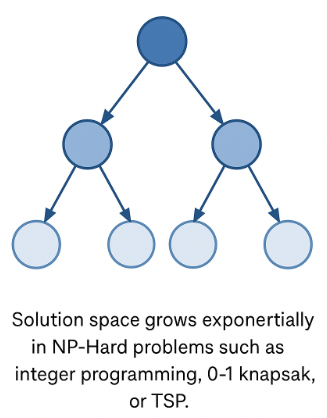
Integer programming problems — where some or all decision variables are constrained to take on integer values — belong to a class of computational problems known as NP-Hard. This means there is no known algorithm that can solve all instances efficiently (i.e., in polynomial time), and the solution space often grows exponentially with problem size. Even seemingly simple problems like the 0-1 knapsack problem or traveling salesman problem (TSP) are NP-Hard when cast as integer programs.
Learn more:
Garey & Johnson, Computers and Intractability: A Guide to the Theory of NP-Completeness, W.H. Freeman, 1979.
Enumeration Methods: Method of Darts#
The Method of Darts is a simple but effective stochastic search technique that bears some resemblance to genetic algorithms. It involves throwing “random darts” — that is, sampling points randomly within the search space — and using the outcomes to guide subsequent throws.
The method begins with a broad scatter of random points across the feasible domain.
Points that yield productive (high-fitness or low-cost) values are retained.
The next round of darts is thrown closer to these productive regions, typically by reducing the variance of the sampling distribution.
Over time, the search becomes more focused, homing in on promising areas of the space.
This adaptive narrowing of the search region makes the Method of Darts a primitive but intuitive global optimization strategy — especially useful when:
The objective function is noisy or discontinuous
Gradients are not available
A lightweight, implementation-flexible approach is preferred
Note
A military equivalent to Method of Darts is Reconissance by Fire :::
import numpy as np

def generate_random_pairs(n,
                          x0_low, x0_high,
                          x1_low, x1_high,
                          x0_target, x1_target,
                          dispersion_1, dispersion_2,
                          distribution='normal',
                          seed=None):
    """
    Generate n 2D points with specified target, dispersion, and distribution.

    Parameters:
        n (int): Number of points
        x0_low, x0_high: Bounds for x0
        x1_low, x1_high: Bounds for x1
        x0_target, x1_target: Mean or mode for each variable
        dispersion_1, dispersion_2: Std dev (for normal), range half-width (for uniform), or std dev (for gamma)
        distribution (str): 'uniform', 'normal', or 'gamma'
        seed (int or None): Optional seed for reproducibility

    Returns:
        list of [x0, x1] pairs
    """
    if seed is not None:
        np.random.seed(seed)

    if distribution == 'uniform':
        x0s = np.random.uniform(x0_target - dispersion_1, x0_target + dispersion_1, n)
        x1s = np.random.uniform(x1_target - dispersion_2, x1_target + dispersion_2, n)

    elif distribution == 'normal':
        x0s = np.random.normal(loc=x0_target, scale=dispersion_1, size=n)
        x1s = np.random.normal(loc=x1_target, scale=dispersion_2, size=n)

    elif distribution == 'gamma':
        # Convert mean and std to shape and scale: mean = shape * scale, std = sqrt(shape * scale^2)
        # Solve for shape and scale given mean (target) and std (dispersion)
        def gamma_params(mean, std):
            shape = (mean / std) ** 2
            scale = std ** 2 / mean
            return shape, scale

        shape0, scale0 = gamma_params(x0_target, dispersion_1)
        shape1, scale1 = gamma_params(x1_target, dispersion_2)

        x0s = np.random.gamma(shape=shape0, scale=scale0, size=n)
        x1s = np.random.gamma(shape=shape1, scale=scale1, size=n)

    else:
        raise ValueError("Unsupported distribution type. Choose from 'uniform', 'normal', 'gamma'.")

    # Clip to bounds
    x0s = np.clip(x0s, x0_low, x0_high)
    x1s = np.clip(x1s, x1_low, x1_high)

    return [[float(x0), float(x1)] for x0, x1 in zip(x0s, x1s)]
samples = generate_random_pairs(
    n=10,
    x0_low=0, x0_high=5,
    x1_low=1, x1_high=6,
    x0_target=2.5, x1_target=3.5,
    dispersion_1=0.8, dispersion_2=1.0,
    distribution='normal',
    seed=42
)

for s in samples:
    print(s)
[2.8973713224089863, 3.0365823071875377]
[2.389388559063052, 3.034270246429743]
[3.018150830480554, 3.741962271566034]
[3.7184238851264206, 1.586719755342202]
[2.3126773002213312, 1.7750821674869672]
[2.3126904344406554, 2.937712470759027]
[3.763370252405913, 2.4871688796655764]
[3.113947783322327, 3.814247332595274]
[2.1244204912520384, 2.591975924478789]
[2.9340480348687716, 2.0876962986647083]
def rosen(x):
    x = np.asarray(x)  # coerce lists to arrays
    return sum(100.0*(x[1:] - x[:-1]**2.0)**2.0 + (1 - x[:-1])**2.0)

z = [1,1]

print(rosen(z))
0.0
# method of darts
samples = generate_random_pairs(
    n=10,
    x0_low=0, x0_high=5,
    x1_low=1, x1_high=6,
    x0_target=2.5, x1_target=3.5,
    dispersion_1=0.8, dispersion_2=1.0,
    distribution='normal',
    seed=42
)

# First Set of Darts
howmany = len(samples)
best = 1e12
best_guess = [0,0]
for i in range(howmany):
    res=rosen(samples[i])
    if res <= best:
        best = res
        best_guess = samples[i]
#    print(samples[i],res)
print(best_guess,best)

# Next Set of Darts
samples = generate_random_pairs(
    n=10,
    x0_low=0.5*best_guess[0], x0_high=2.0*best_guess[0],
    x1_low=0.5*best_guess[0], x1_high=2.0*best_guess[0],
    x0_target=best_guess[0], x1_target=best_guess[1],
    dispersion_1=0.8, dispersion_2=1.0,
    distribution='normal',
    seed=42
)
howmany = len(samples)
#best = 1e12
#best_guess = [0,0]
for i in range(howmany):
    res=rosen(samples[i])
    if res <= best:
        best = res
        best_guess = samples[i]
#    print(samples[i],res)
print(best_guess,best)

# Next Set of Darts
samples = generate_random_pairs(
    n=10,
    x0_low=0.5*best_guess[0], x0_high=2.0*best_guess[0],
    x1_low=0.5*best_guess[0], x1_high=2.0*best_guess[0],
    x0_target=best_guess[0], x1_target=best_guess[1],
    dispersion_1=2.0*best_guess[0]-0.5*best_guess[0], dispersion_2=2.0*best_guess[1]-0.5*best_guess[1],
    distribution='normal',
    seed=42
)
howmany = len(samples)
#best = 1e12
#best_guess = [0,0]
for i in range(howmany):
    res=rosen(samples[i])
    if res <= best:
        best = res
        best_guess = samples[i]
#    print(samples[i],res)
print(best_guess,best)
[2.1244204912520384, 2.591975924478789] 370.3600779015173
[1.7488409825040767, 1.6839518489575784] 189.48384513902653
[0.8744204912520384, 0.8744204912520384] 1.221578355902027
[0.6930687840229477, 0.4372102456260192] 0.2802617757996684
import numpy as np

def rosen(x):
    """The Rosenbrock function"""
    x = np.asarray(x)
    return sum(100.0*(x[1:] - x[:-1]**2.0)**2.0 + (1 - x[:-1])**2.0)

def dart_search(n_darts, x0_bounds, x1_bounds, x0_target, x1_target,
                dispersion_1, dispersion_2, distribution='normal', seed=None):
    """Generate random samples and evaluate them using the Rosenbrock function."""
    samples = generate_random_pairs(
        n=n_darts,
        x0_low=x0_bounds[0], x0_high=x0_bounds[1],
        x1_low=x1_bounds[0], x1_high=x1_bounds[1],
        x0_target=x0_target, x1_target=x1_target,
        dispersion_1=dispersion_1, dispersion_2=dispersion_2,
        distribution=distribution,
        seed=seed
    )

    best_val = 1e12
#    best_point = [0, 0]
    best_point = [x0_target, x1_target]
    worst_point = best_point
    worst_val = 1e-9
    for s in samples:
        res = rosen(s)
        if res < best_val:
            best_val = res
            best_point = s
        if res > worst_val:
            worst_val = res
            worst_point = s
    return best_point, best_val, worst_point, worst_val

def repeat_dart_cycles(n_cycles=4, darts_per_cycle=10,
                       initial_bounds=((-2, 2), (-1, 3)),
                       initial_target=(2.5, 3.5),
                       initial_dispersion=(0.8, 1.0),
                       distribution='normal',
                       verbose=True):
    """Repeat dart throws and refine the guess with each cycle."""
    best_guess = initial_target
    best_value = 1e12
    worst_guess = initial_target
    worst_value = 1e-9

    string_of_darts = []

    for cycle in range(n_cycles):
        x0_bounds = (0.9 * best_guess[0], 1.1 * best_guess[0])
        x1_bounds = (0.9 * best_guess[1], 1.1 * best_guess[1])
        dispersion_1 = 0.5*(x0_bounds[1] - x0_bounds[0])
        dispersion_2 = 0.5*(x1_bounds[1] - x1_bounds[0])

        best_guess, best_value, worst_guess, worst_val = dart_search(
            n_darts=darts_per_cycle,
            x0_bounds=x0_bounds,
            x1_bounds=x1_bounds,
            x0_target=best_guess[0],
            x1_target=best_guess[1],
            dispersion_1=dispersion_1,
            dispersion_2=dispersion_2,
            distribution=distribution,
            seed=42
        )
        if verbose:
            print(f"Cycle {cycle+1}: best_guess = [ {best_guess[0]:.6f}, {best_guess[1]:.6f}],  best_value = {best_value:.6f}")
        string_of_darts.append([best_guess[0],best_guess[1],best_value])
    return best_guess, best_value, worst_guess, worst_val, string_of_darts
best_pt, best_val , worst_pt, worst_val , string_of_darts = repeat_dart_cycles(
    n_cycles=9,
    darts_per_cycle=900,
    initial_bounds=((-2, 2), (-2, 2)),
    initial_target=(0.999621, 0.999134),
    initial_dispersion=(1.0, 1.0),
    distribution='gamma'
)
Cycle 1: best_guess = [ 1.002252, 1.004188],  best_value = 0.000015
Cycle 2: best_guess = [ 1.004889, 1.009268],  best_value = 0.000052
Cycle 3: best_guess = [ 1.007534, 1.014374],  best_value = 0.000113
Cycle 4: best_guess = [ 0.991979, 0.984131],  best_value = 0.000066
Cycle 5: best_guess = [ 0.994589, 0.989109],  best_value = 0.000030
Cycle 6: best_guess = [ 0.997207, 0.994113],  best_value = 0.000017
Cycle 7: best_guess = [ 0.999831, 0.999142],  best_value = 0.000027
Cycle 8: best_guess = [ 1.002462, 1.004196], best_value = 0.000060
Cycle 9: best_guess = [ 1.005100, 1.009276], best_value = 0.000116
print(string_of_darts)
[[1.0022516200544278, 1.0041884106440682, np.float64(1.5303346374449118e-05)], [1.004889162894462, 1.009268390498031, np.float64(5.2402343456230996e-05)], [1.0075336467382263, 1.0143740689111922, np.float64(0.00011300289298032522)], [0.991978904279407, 0.9841307727517556, np.float64(6.551794204747527e-05)], [0.994589413261478, 0.9891092851964847, np.float64(3.0250904600404742e-05)], [0.9972067921045068, 0.9941129828979383, np.float64(1.7313271213906414e-05)], [0.9998310588873391, 0.9991419932630805, np.float64(2.708446092258635e-05)], [1.0024622317363978, 1.0041964443434008, np.float64(5.995018148276627e-05)], [1.005100328825807, 1.0092764648381742, np.float64(0.00011630253022035773)]]
worst_val
np.float64(9.756754729127907)