Semester Project - in Python
this section is under development, students should continue to use ModelMuse, the python is not particularly intuitive.
Here is a python approach to access MODFLOW6 using Jupyter Notebook running an ipython kernel.
There was an installation step for FloPy and manual compilation of MODFLOW6 to run on a Raspberry Pi (to make the notes) Use the ! get-modflow method in the notes for intel-based machines.
Step 1
Build MODFLOW6 on server (I used a raspberry pi, the install notes show how to get binaries directly for intel machines)
Convert example problem into the 5-layer case to understand the model syntax.
Use a default recharge package from modflow6-examples.readthedocs.io
Use a wellfield package to include wells (adjust pumpage as needed to activate/deactivate)
import warnings
warnings.filterwarnings('ignore')

# Now attempt an example
import os
import numpy as np
import matplotlib.pyplot as plt
import flopy

name = "project1-1_mf6"
h1 = 100
h2 = 90
hriv = -25 #river elevation reference to top
Nlay = 5 #number layers
Nrow = 24 #number rows
Ncol = 10 #number columns
LR = Nrow*1000.0 # length in row direction
LC = Ncol*1000.0 # length in column direction
H = 175.0 # aquifer thickness
k = 20.0*365 # hydraulic condictivity

sim = flopy.mf6.MFSimulation(
    sim_name=name, exe_name="/home/sensei/ce-4363-webroot/ModflowExperimental/mf6-arm/mf6", version="mf6", sim_ws="/home/sensei/ce-4363-webroot/ModflowExperimental/mf6-arm/project1-1"
)

tdis = flopy.mf6.ModflowTdis(
    sim, pname="tdis", time_units="YEARS", nper=1, perioddata=[(1.0, 1, 1.0)]
)

ims = flopy.mf6.ModflowIms(sim, pname="ims", complexity="SIMPLE")

model_nam_file = "{}.nam".format(name)
gwf = flopy.mf6.ModflowGwf(sim, modelname=name, model_nam_file=model_nam_file)

#bot = np.linspace(-H / Nlay, -H, Nlay)
bot = np.array([-50,-95,-100,-150,-175])
#print(bot)
delrow = LR/Nrow
delcol = LC/Ncol
dis = flopy.mf6.ModflowGwfdis(
    gwf,
    nlay=Nlay,
    nrow=Nrow,
    ncol=Ncol,
    delr=delrow,
    delc=delcol,
    top=0.0,
    botm=bot,
)

#start heads
start = hriv * np.ones((Nlay, Nrow, Ncol))
ic = flopy.mf6.ModflowGwfic(gwf, pname="ic", strt=start)

npf = flopy.mf6.ModflowGwfnpf(gwf, icelltype=1, k=k, save_flows=True)

# create constant head boundaries
chd_rec = []
#chd_rec.append(((0, 19, 5), hriv))
for layer in range(0, 1):
    for col in range(0,Ncol):
        chd_rec.append(((layer, 8, col), hriv))

chd = flopy.mf6.ModflowGwfchd(
    gwf,
    maxbound=len(chd_rec),
    stress_period_data=chd_rec,
    save_flows=True,
)

# ### Create the well (`WEL`) Package
#
# Add a well in model layer 5.

wel_rec = []
wel_rec.append((0, 21, 5, -1)) #wellfieldA-upper
wel_rec.append((1, 21, 5, -1)) #wellfieldA-lower
wel_rec.append((3, 14, 6, -1)) #wellfieldB-upper
wel_rec.append((4, 14, 6, -1)) #wellfieldB-lower
wel_rec.append((3, 4, 6, -1)) #wellfieldC-upper
wel_rec.append((4, 4, 6, -1)) #wellfieldC-lower
#wel_rec = [(4, 21, 5, -1000)]
wel = flopy.mf6.ModflowGwfwel(
    gwf,
    stress_period_data=wel_rec,
)

iper = 0
ra = chd.stress_period_data.get_data(key=iper)
#ra

flopy.mf6.ModflowGwfrcha(gwf, recharge=2.5e-1)

# Create the output control (`OC`) Package
headfile = "{}.hds".format(name)
head_filerecord = [headfile]
budgetfile = "{}.cbb".format(name)
budget_filerecord = [budgetfile]
saverecord = [("HEAD", "ALL"), ("BUDGET", "ALL")]
printrecord = [("HEAD", "LAST")]
oc = flopy.mf6.ModflowGwfoc(
    gwf,
    saverecord=saverecord,
    head_filerecord=head_filerecord,
    budget_filerecord=budget_filerecord,
    printrecord=printrecord,
)

sim.write_simulation()


import tracemalloc
tracemalloc.start() # this is to suppress an asyncronous warning

# attempt to run the model, will see if binary loaded OK
success, buff = sim.run_simulation()
if not success:
    raise Exception("MODFLOW 6 did not terminate normally.")

current, peak = tracemalloc.get_traced_memory()
print("Current memory usage is %d bytes; peak was %d bytes" % (current, peak))
writing simulation...
  writing simulation name file...
  writing simulation tdis package...
  writing ims package ims...
  writing model project1-1_mf6...
    writing model name file...
    writing package dis...
    writing package ic...
    writing package npf...
    writing package chd_0...
    writing package wel_0...
INFORMATION: maxbound in ('gwf6', 'wel', 'dimensions') changed to 6 based on size of stress_period_data
    writing package rcha_0...
    writing package oc...
FloPy is using the following executable to run the model: /home/sensei/ce-4363-webroot/ModflowExperimental/mf6-arm/mf6
                                   MODFLOW 6
                U.S. GEOLOGICAL SURVEY MODULAR HYDROLOGIC MODEL
                        VERSION 6.4.1 Release 12/09/2022

         MODFLOW 6 compiled Apr 16 2023 18:27:14 with GCC version 9.4.0

This software has been approved for release by the U.S. Geological
Survey (USGS). Although the software has been subjected to rigorous
review, the USGS reserves the right to update the software as needed
pursuant to further analysis and review. No warranty, expressed or
implied, is made by the USGS or the U.S. Government as to the
functionality of the software and related material nor shall the
fact of release constitute any such warranty. Furthermore, the
software is released on condition that neither the USGS nor the U.S.
Government shall be held liable for any damages resulting from its
authorized or unauthorized use. Also refer to the USGS Water
Resources Software User Rights Notice for complete use, copyright,
and distribution information.


 Run start date and time (yyyy/mm/dd hh:mm:ss): 2024/02/01 17:47:32

 Writing simulation list file: mfsim.lst
 Using Simulation name file: mfsim.nam

    Solving:  Stress period:     1    Time step:     1

 Run end date and time (yyyy/mm/dd hh:mm:ss): 2024/02/01 17:47:32
 Elapsed run time:  0.059 Seconds

 Normal termination of simulation.
Current memory usage is 8608 bytes; peak was 59207 bytes
# now attempt to postprocess
h = gwf.output.head().get_data(kstpkper=(0, 0))
x = np.linspace(0, LC, Ncol )
y = np.linspace(0, LR, Nrow )
y = y[::-1]
vmin, vmax = -175.0, 0.0
contour_intervals = np.arange(-175, 10, 1.0)
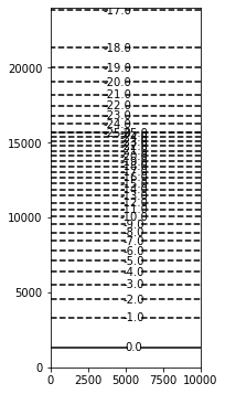
# ### Plot a Map of Layer 1
fig = plt.figure(figsize=(6, 6))
ax = fig.add_subplot(1, 1, 1, aspect="equal")
c = ax.contour(x, y, h[0], contour_intervals, colors="black")
plt.clabel(c, fmt="%2.1f")
#print(contour_intervals)
/opt/jupyterhub/lib/python3.8/site-packages/ipykernel/ipkernel.py:287: DeprecationWarning: `should_run_async` will not call `transform_cell` automatically in the future. Please pass the result to `transformed_cell` argument and any exception that happen during thetransform in `preprocessing_exc_tuple` in IPython 7.17 and above.
  and should_run_async(code)
<a list of 35 text.Text objects>
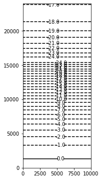
# ### Plot a Map of Layer 5

fig = plt.figure(figsize=(6, 6))
ax = fig.add_subplot(1, 1, 1, aspect="equal")
c = ax.contour(x, y, h[4], contour_intervals, colors="black")
plt.clabel(c, fmt="%2.1f")
/opt/jupyterhub/lib/python3.8/site-packages/ipykernel/ipkernel.py:287: DeprecationWarning: `should_run_async` will not call `transform_cell` automatically in the future. Please pass the result to `transformed_cell` argument and any exception that happen during thetransform in `preprocessing_exc_tuple` in IPython 7.17 and above.
  and should_run_async(code)
<a list of 33 text.Text objects>
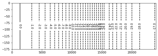
# now try a slice
# ### Plot a Cross-section along column 6

z = np.linspace(-175, 0 , Nlay)
fig = plt.figure(figsize=(9, 3))
ax = fig.add_subplot(1, 1, 1, aspect="auto")
c = ax.contour(y, z, h[:, :,5], contour_intervals, colors="black")
plt.clabel(c, fmt="%1.1f")
/opt/jupyterhub/lib/python3.8/site-packages/ipykernel/ipkernel.py:287: DeprecationWarning: `should_run_async` will not call `transform_cell` automatically in the future. Please pass the result to `transformed_cell` argument and any exception that happen during thetransform in `preprocessing_exc_tuple` in IPython 7.17 and above.
  and should_run_async(code)
<a list of 33 text.Text objects>
Step 2 (and beyond)
Ok seems to be a running model, 5 layers, with a constant head boundary and recharge.
The next step is to activete the wellfields, then figure out how to define spatial varying \(K\) for each layer, then spatial varying \(S\) for each layer without breaking the model. Then turn into transient simulator, and run the time-varying cases.
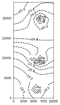
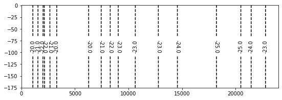
Next case is with wellfield C at the lower bound of pumpage rate. Flow is towards river cells - so feasible as per problem statement.
import warnings
warnings.filterwarnings('ignore')

# Now attempt an example
import os
import numpy as np
import matplotlib.pyplot as plt
import flopy

name = "project1-1_mf6"
h1 = 100
h2 = 90
hriv = -25 #river elevation reference to bottom
Nlay = 5 #number layers
Nrow = 24 #number rows
Ncol = 10 #number columns
LR = Nrow*1000.0 # length in row direction
LC = Ncol*1000.0 # length in column direction
H = 175.0 # aquifer thickness
k = 20.0*365 # hydraulic condictivity

sim = flopy.mf6.MFSimulation(
    sim_name=name, exe_name="/home/sensei/ce-4363-webroot/ModflowExperimental/mf6-arm/mf6", version="mf6", sim_ws="/home/sensei/ce-4363-webroot/ModflowExperimental/mf6-arm/project1-1"
)

tdis = flopy.mf6.ModflowTdis(
    sim, pname="tdis", time_units="YEARS", nper=1, perioddata=[(1.0, 1, 1.0)]
)

ims = flopy.mf6.ModflowIms(sim, pname="ims", complexity="SIMPLE")

model_nam_file = "{}.nam".format(name)
gwf = flopy.mf6.ModflowGwf(sim, modelname=name, model_nam_file=model_nam_file)

#bot = np.linspace(-H / Nlay, -H, Nlay)
bot = np.array([-50,-95,-100,-150,-175])
#bot = np.array([125,80,75,25,0])
#print(bot)
delrow = LR/Nrow
delcol = LC/Ncol
dis = flopy.mf6.ModflowGwfdis(
    gwf,
    nlay=Nlay,
    nrow=Nrow,
    ncol=Ncol,
    delr=delrow,
    delc=delcol,
    top=0.0,
    botm=bot,
)

#start heads
start = hriv * np.ones((Nlay, Nrow, Ncol))
ic = flopy.mf6.ModflowGwfic(gwf, pname="ic", strt=start)

npf = flopy.mf6.ModflowGwfnpf(gwf, icelltype=1, k=k, save_flows=True)

# create constant head boundaries
chd_rec = []
#chd_rec.append(((0, 19, 5), hriv))
for layer in range(0, 1):
    for col in range(0,Ncol):
        chd_rec.append(((layer, 8, col), hriv))

chd = flopy.mf6.ModflowGwfchd(
    gwf,
    maxbound=len(chd_rec),
    stress_period_data=chd_rec,
    save_flows=True,
)

# ### Create the well (`WEL`) Package
#
# Add a well in model layer 5.

wel_rec = []
wel_rec.append((0, 21, 5, -5.0e06)) #wellfieldA-upper
wel_rec.append((1, 21, 5, -5.0e06)) #wellfieldA-lower
wel_rec.append((3, 14, 6, -8.0e06)) #wellfieldB-upper
wel_rec.append((4, 14, 6, -8.0e06)) #wellfieldB-lower
wel_rec.append((3, 4, 6, -7.5e06*1)) #wellfieldC-upper
wel_rec.append((4, 4, 6, -7.5e06*1)) #wellfieldC-lower
#wel_rec = [(4, 21, 5, -1000)]
wel = flopy.mf6.ModflowGwfwel(
    gwf,
    stress_period_data=wel_rec,
)

iper = 0
ra = chd.stress_period_data.get_data(key=iper)
#ra

flopy.mf6.ModflowGwfrcha(gwf, recharge=2.5e-1)

# Create the output control (`OC`) Package
headfile = "{}.hds".format(name)
head_filerecord = [headfile]
budgetfile = "{}.cbb".format(name)
budget_filerecord = [budgetfile]
saverecord = [("HEAD", "ALL"), ("BUDGET", "ALL")]
printrecord = [("HEAD", "LAST")]
oc = flopy.mf6.ModflowGwfoc(
    gwf,
    saverecord=saverecord,
    head_filerecord=head_filerecord,
    budget_filerecord=budget_filerecord,
    printrecord=printrecord,
)

sim.write_simulation()


import tracemalloc
tracemalloc.start() # this is to suppress an asyncronous warning

# attempt to run the model, will see if binary loaded OK
success, buff = sim.run_simulation()
if not success:
    raise Exception("MODFLOW 6 did not terminate normally.")

current, peak = tracemalloc.get_traced_memory()
print("Current memory usage is %d bytes; peak was %d bytes" % (current, peak))
/opt/jupyterhub/lib/python3.8/site-packages/ipykernel/ipkernel.py:287: DeprecationWarning: `should_run_async` will not call `transform_cell` automatically in the future. Please pass the result to `transformed_cell` argument and any exception that happen during thetransform in `preprocessing_exc_tuple` in IPython 7.17 and above.
  and should_run_async(code)
writing simulation...
  writing simulation name file...
  writing simulation tdis package...
  writing ims package ims...
  writing model project1-1_mf6...
    writing model name file...
    writing package dis...
    writing package ic...
    writing package npf...
    writing package chd_0...
    writing package wel_0...
INFORMATION: maxbound in ('gwf6', 'wel', 'dimensions') changed to 6 based on size of stress_period_data
    writing package rcha_0...
    writing package oc...
FloPy is using the following executable to run the model: /home/sensei/ce-4363-webroot/ModflowExperimental/mf6-arm/mf6
                                   MODFLOW 6
                U.S. GEOLOGICAL SURVEY MODULAR HYDROLOGIC MODEL
                        VERSION 6.4.1 Release 12/09/2022

         MODFLOW 6 compiled Apr 16 2023 18:27:14 with GCC version 9.4.0

This software has been approved for release by the U.S. Geological
Survey (USGS). Although the software has been subjected to rigorous
review, the USGS reserves the right to update the software as needed
pursuant to further analysis and review. No warranty, expressed or
implied, is made by the USGS or the U.S. Government as to the
functionality of the software and related material nor shall the
fact of release constitute any such warranty. Furthermore, the
software is released on condition that neither the USGS nor the U.S.
Government shall be held liable for any damages resulting from its
authorized or unauthorized use. Also refer to the USGS Water
Resources Software User Rights Notice for complete use, copyright,
and distribution information.


 Run start date and time (yyyy/mm/dd hh:mm:ss): 2024/02/01 17:47:41

 Writing simulation list file: mfsim.lst
 Using Simulation name file: mfsim.nam

    Solving:  Stress period:     1    Time step:     1

 Run end date and time (yyyy/mm/dd hh:mm:ss): 2024/02/01 17:47:41
 Elapsed run time:  0.056 Seconds

 Normal termination of simulation.
Current memory usage is 10206220 bytes; peak was 10259387 bytes
# now attempt to postprocess
h = gwf.output.head().get_data(kstpkper=(0, 0))
x = np.linspace(0, LC, Ncol )
y = np.linspace(0, LR, Nrow )
y = y[::-1]
vmin, vmax = -175.0, 0.0
contour_intervals = np.arange(-175, 10, 1.0)

# ### Plot a Map of Layer 1

fig = plt.figure(figsize=(6, 6))
ax = fig.add_subplot(1, 1, 1, aspect="equal")
c = ax.contour(x, y, h[0], contour_intervals, colors="black")
plt.clabel(c, fmt="%2.1f")
#print(contour_intervals)
<a list of 20 text.Text objects>
# ### Plot a Map of Layer 5

fig = plt.figure(figsize=(6, 6))
ax = fig.add_subplot(1, 1, 1, aspect="equal")
c = ax.contour(x, y, h[4], contour_intervals, colors="black")
plt.clabel(c, fmt="%2.1f")
<a list of 18 text.Text objects>
# now try a slice
# ### Plot a Cross-section along column 6

z = np.linspace(-175, 1 , Nlay)
fig = plt.figure(figsize=(9, 3))
ax = fig.add_subplot(1, 1, 1, aspect="auto")
c = ax.contour(y, z, h[:, :,5], contour_intervals, colors="black")
plt.clabel(c, fmt="%1.1f")
<a list of 17 text.Text objects>
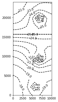
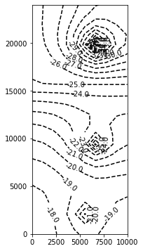
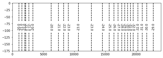
Wellfield C at maximum target rate, notice in the slice, that there is flow from the river cells to the north, so this is too much pumpage as per the problem statement.
import warnings
warnings.filterwarnings('ignore')

# Now attempt an example
import os
import numpy as np
import matplotlib.pyplot as plt
import flopy

name = "project1-1_mf6"
h1 = 100
h2 = 90
hriv = -25 #river elevation reference to bottom
Nlay = 5 #number layers
Nrow = 24 #number rows
Ncol = 10 #number columns
LR = Nrow*1000.0 # length in row direction
LC = Ncol*1000.0 # length in column direction
H = 175.0 # aquifer thickness
k = 20.0*365 # hydraulic condictivity

sim = flopy.mf6.MFSimulation(
    sim_name=name, exe_name="/home/sensei/ce-4363-webroot/ModflowExperimental/mf6-arm/mf6", version="mf6", sim_ws="/home/sensei/ce-4363-webroot/ModflowExperimental/mf6-arm/project1-1"
)

tdis = flopy.mf6.ModflowTdis(
    sim, pname="tdis", time_units="YEARS", nper=1, perioddata=[(1.0, 1, 1.0)]
)

ims = flopy.mf6.ModflowIms(sim, pname="ims", complexity="SIMPLE")

model_nam_file = "{}.nam".format(name)
gwf = flopy.mf6.ModflowGwf(sim, modelname=name, model_nam_file=model_nam_file)

#bot = np.linspace(-H / Nlay, -H, Nlay)
bot = np.array([-50,-95,-100,-150,-175])
#bot = np.array([125,80,75,25,0])
#print(bot)
delrow = LR/Nrow
delcol = LC/Ncol
dis = flopy.mf6.ModflowGwfdis(
    gwf,
    nlay=Nlay,
    nrow=Nrow,
    ncol=Ncol,
    delr=delrow,
    delc=delcol,
    top=0.0,
    botm=bot,
)

#start heads
start = hriv * np.ones((Nlay, Nrow, Ncol))
ic = flopy.mf6.ModflowGwfic(gwf, pname="ic", strt=start)

npf = flopy.mf6.ModflowGwfnpf(gwf, icelltype=1, k=k, save_flows=True)

# create constant head boundaries
chd_rec = []
#chd_rec.append(((0, 19, 5), hriv))
for layer in range(0, 1):
    for col in range(0,Ncol):
        chd_rec.append(((layer, 8, col), hriv))

chd = flopy.mf6.ModflowGwfchd(
    gwf,
    maxbound=len(chd_rec),
    stress_period_data=chd_rec,
    save_flows=True,
)

# ### Create the well (`WEL`) Package
#
# Add a well in model layer 5.

wel_rec = []
wel_rec.append((0, 21, 5, -5.0e06)) #wellfieldA-upper
wel_rec.append((1, 21, 5, -5.0e06)) #wellfieldA-lower
wel_rec.append((3, 14, 6, -8.0e06)) #wellfieldB-upper
wel_rec.append((4, 14, 6, -8.0e06)) #wellfieldB-lower
wel_rec.append((3, 4, 6, -7.5e06*2)) #wellfieldC-upper
wel_rec.append((4, 4, 6, -7.5e06*2)) #wellfieldC-lower
#wel_rec = [(4, 21, 5, -1000)]
wel = flopy.mf6.ModflowGwfwel(
    gwf,
    stress_period_data=wel_rec,
)

iper = 0
ra = chd.stress_period_data.get_data(key=iper)
#ra

flopy.mf6.ModflowGwfrcha(gwf, recharge=2.5e-1)

# Create the output control (`OC`) Package
headfile = "{}.hds".format(name)
head_filerecord = [headfile]
budgetfile = "{}.cbb".format(name)
budget_filerecord = [budgetfile]
saverecord = [("HEAD", "ALL"), ("BUDGET", "ALL")]
printrecord = [("HEAD", "LAST")]
oc = flopy.mf6.ModflowGwfoc(
    gwf,
    saverecord=saverecord,
    head_filerecord=head_filerecord,
    budget_filerecord=budget_filerecord,
    printrecord=printrecord,
)

sim.write_simulation()


import tracemalloc
tracemalloc.start() # this is to suppress an asyncronous warning

# attempt to run the model, will see if binary loaded OK
success, buff = sim.run_simulation()
if not success:
    raise Exception("MODFLOW 6 did not terminate normally.")

current, peak = tracemalloc.get_traced_memory()
print("Current memory usage is %d bytes; peak was %d bytes" % (current, peak))
writing simulation...
  writing simulation name file...
  writing simulation tdis package...
  writing ims package ims...
  writing model project1-1_mf6...
    writing model name file...
    writing package dis...
    writing package ic...
    writing package npf...
    writing package chd_0...
    writing package wel_0...
INFORMATION: maxbound in ('gwf6', 'wel', 'dimensions') changed to 6 based on size of stress_period_data
    writing package rcha_0...
    writing package oc...
FloPy is using the following executable to run the model: /home/sensei/ce-4363-webroot/ModflowExperimental/mf6-arm/mf6
                                   MODFLOW 6
                U.S. GEOLOGICAL SURVEY MODULAR HYDROLOGIC MODEL
                        VERSION 6.4.1 Release 12/09/2022

         MODFLOW 6 compiled Apr 16 2023 18:27:14 with GCC version 9.4.0

This software has been approved for release by the U.S. Geological
Survey (USGS). Although the software has been subjected to rigorous
review, the USGS reserves the right to update the software as needed
pursuant to further analysis and review. No warranty, expressed or
implied, is made by the USGS or the U.S. Government as to the
functionality of the software and related material nor shall the
fact of release constitute any such warranty. Furthermore, the
software is released on condition that neither the USGS nor the U.S.
Government shall be held liable for any damages resulting from its
authorized or unauthorized use. Also refer to the USGS Water
Resources Software User Rights Notice for complete use, copyright,
and distribution information.


 Run start date and time (yyyy/mm/dd hh:mm:ss): 2024/02/01 17:47:48

 Writing simulation list file: mfsim.lst
 Using Simulation name file: mfsim.nam

    Solving:  Stress period:     1    Time step:     1

 Run end date and time (yyyy/mm/dd hh:mm:ss): 2024/02/01 17:47:48
 Elapsed run time:  0.062 Seconds

 Normal termination of simulation.
Current memory usage is 18868537 bytes; peak was 18921973 bytes
# now attempt to postprocess
h = gwf.output.head().get_data(kstpkper=(0, 0))
x = np.linspace(0, LC, Ncol )
y = np.linspace(0, LR, Nrow )
y = y[::-1]
vmin, vmax = -175.0, 0.0
contour_intervals = np.arange(-175, 10, 1.0)

# ### Plot a Map of Layer 1

fig = plt.figure(figsize=(6, 6))
ax = fig.add_subplot(1, 1, 1, aspect="equal")
c = ax.contour(x, y, h[0], contour_intervals, colors="black")
plt.clabel(c, fmt="%2.1f")
#print(contour_intervals)
<a list of 24 text.Text objects>

# ### Plot a Map of Layer 5

fig = plt.figure(figsize=(6, 6))
ax = fig.add_subplot(1, 1, 1, aspect="equal")
c = ax.contour(x, y, h[4], contour_intervals, colors="black")
plt.clabel(c, fmt="%2.1f")
<a list of 24 text.Text objects>
# now try a slice
# ### Plot a Cross-section along column 6

z = np.linspace(-175, 1 , Nlay)
fig = plt.figure(figsize=(9, 3))
ax = fig.add_subplot(1, 1, 1, aspect="auto")
c = ax.contour(y, z, h[:, :,5], contour_intervals, colors="black")
plt.clabel(c, fmt="%1.1f")
<a list of 25 text.Text objects>
Step 3
Spatial varying K
Add storage
Turn into transient