MODFLOW Python Interface Examples
A way to access MODFLOW using Python and Jupyter Notebooks is avaliable at
FloPy: Python Package for Creating, Running, and Post-Processing MODFLOW-Based Models
The PDF link below shows the installation and an example run on the AWS server.
MODFLOW on a Jupyter Server - notes
Examples
The remainder of this section is worked examples using FLOPY and MODFLOW6 installed on a aarch-64 computer. x86-... architectures should use the ! get-modflow method to download (in near real time) current binaries
Project Example
The figure below is a map and cross section of an aquifer system.
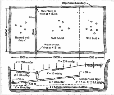
Two well fields operate in the area; well field A pumping \(10 \times 10^{6} \frac{m^3}{yr}\) and a well field B pumping \(16 \times 10^{6} \frac{m^3}{yr}\) All the intake screens in well field B are below the semipervious layer. A new wellfield, C is planned, with an annual withdrawl of \(15 \times 10^{6} \frac{m^3}{yr}\) and, if possible, up to \(25 \times 10^{6} \frac{m^3}{yr}\).
Use MODFLOW to evaluate the feasibility of the proposed pumping rates for well field C. The river itself should not serve as a water source because the water rights are already apportioned (i.e. someone else owns the water).
The plan view layout and the 5-layer conceptualization are shown below.
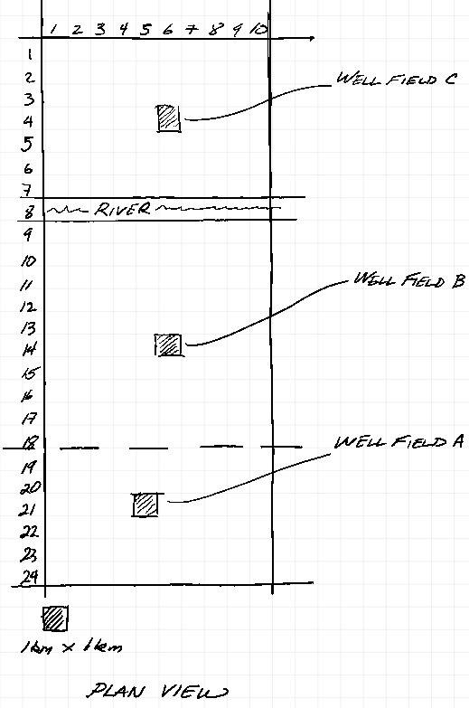
The vertical discritization used is a 5-layer conceptualization to mimic the aquifer system.
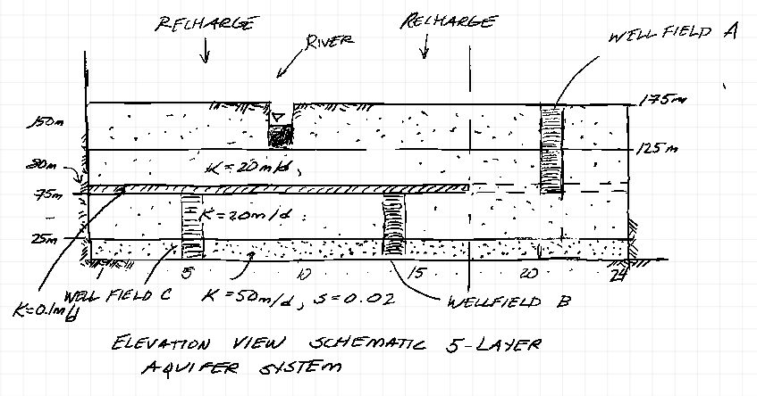
The upper aquifer layer is unconfined and the river is represented using constant head boundaries. The next layer is a confined/unconfined layer and is where the well field A wells are screened (65-125 meters). The aquitard is a thin layer from (60-65 meters) with spatially varying hydraulic conductivity. The lower aquifers are represented as confined in MODFLOW, with well screens as shown.
Below we use MODFLOW to produce:
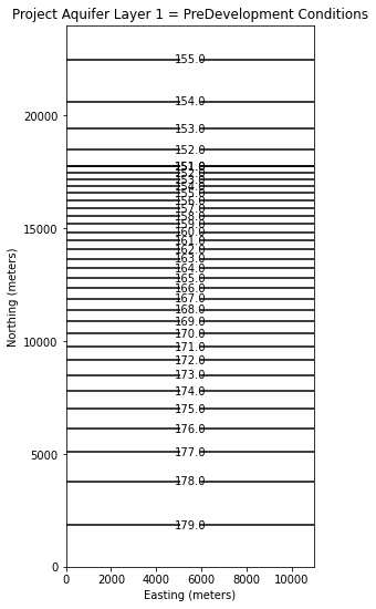
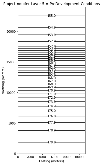
An equilibrium head distribution for all 5 aquifer layers in this system, with zero pumping in all wellfields. This is a pre-development case (recharge only).
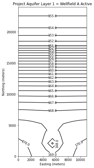
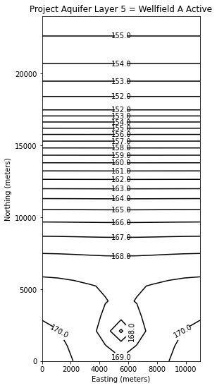
An equilibrium head distribution for the system with only Wellfield A active (assuming 30 years is long enough to reach equilibrium).
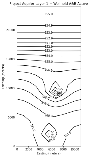
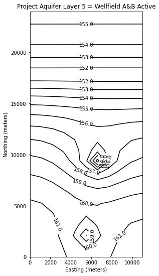
An equilibrium head distribution for the system with Wellfields A and B active at the prescribed rates. (Again assuming 30 years is long enough to reach equilibrium).
An equilibrium head distribution for the system with Wellfields A and B active at the prescribed rates; Wellfield C is active, but rate is increased by trial-error until gradient from river indicates flow into the aquifer.
import warnings
warnings.filterwarnings('ignore')
import os
import numpy as np
import matplotlib.pyplot as plt
import flopy
#dir(flopy.mf6)
/opt/jupyterhub/lib/python3.8/site-packages/ipykernel/ipkernel.py:287: DeprecationWarning: `should_run_async` will not call `transform_cell` automatically in the future. Please pass the result to `transformed_cell` argument and any exception that happen during thetransform in `preprocessing_exc_tuple` in IPython 7.17 and above.
  and should_run_async(code)
# Workspace and Executibles
binary = "/home/sensei/ce-4363-webroot/ModflowExperimental/mf6-arm/mf6"  # location on MY computer of the compiled modflow program
workarea = "/home/sensei/ce-4363-webroot/ModflowExperimental/mf6-arm/project_1" # location on MY computer to store files this example (directory must already exist)

# Set Simulation Name
name = "project_1"
#modelname=name

##### FLOPY Build simulation framework ####
sim = flopy.mf6.MFSimulation(
    sim_name=name, exe_name=binary, version="mf6", sim_ws=workarea
)
/opt/jupyterhub/lib/python3.8/site-packages/ipykernel/ipkernel.py:287: DeprecationWarning: `should_run_async` will not call `transform_cell` automatically in the future. Please pass the result to `transformed_cell` argument and any exception that happen during thetransform in `preprocessing_exc_tuple` in IPython 7.17 and above.
  and should_run_async(code)
# Set Time Structure
Time_Units="YEARS"

# Multiple stress periods
nper = 4 # how many periods
# perlen = how long each one in problem time units
# nstp =  how many steps in each stress period
# tsmult = time step multiplier
# perioddata = [(perlen,nstp,tsmult),(perlen,nstp,tsmult),(perlen,nstp,tsmult) ... repeat for each stress period]

perioddata = [(30.0,30,1),(30.0,30,1),(30.0,30,1),(30.0,30,1)]

##### FLOPY Build time framework ##########
tdis = flopy.mf6.ModflowTdis(
    sim, pname="tdis", time_units=Time_Units, nper=nper, perioddata=perioddata,
)
/opt/jupyterhub/lib/python3.8/site-packages/ipykernel/ipkernel.py:287: DeprecationWarning: `should_run_async` will not call `transform_cell` automatically in the future. Please pass the result to `transformed_cell` argument and any exception that happen during thetransform in `preprocessing_exc_tuple` in IPython 7.17 and above.
  and should_run_async(code)
# Set Iterative Model Solution (choose solver parameters)
# about IMS see: https://water.usgs.gov/nrp/gwsoftware/ModelMuse/Help/sms_sparse_matrix_solution_pac.htm
# using defaults see: https://flopy.readthedocs.io/en/3.3.2/source/flopy.mf6.modflow.mfims.html

##### FLOPY Build IMS framework ###########
ims = flopy.mf6.ModflowIms(sim, pname="ims", complexity="SIMPLE")
/opt/jupyterhub/lib/python3.8/site-packages/ipykernel/ipkernel.py:287: DeprecationWarning: `should_run_async` will not call `transform_cell` automatically in the future. Please pass the result to `transformed_cell` argument and any exception that happen during thetransform in `preprocessing_exc_tuple` in IPython 7.17 and above.
  and should_run_async(code)
# Set Model Name (using same base name as the simulation)
model_nam_file = "{}.nam".format(name)

##### FLOPY Build Model Name framework ####
gwf = flopy.mf6.ModflowGwf(sim, modelname=name, model_nam_file=model_nam_file)
/opt/jupyterhub/lib/python3.8/site-packages/ipykernel/ipkernel.py:287: DeprecationWarning: `should_run_async` will not call `transform_cell` automatically in the future. Please pass the result to `transformed_cell` argument and any exception that happen during thetransform in `preprocessing_exc_tuple` in IPython 7.17 and above.
  and should_run_async(code)
# Define The Grid
Nlay = 5 #number layers
Nrow = 24 #number rows
Ncol = 11 #number columns
# Define distances and elevations
delrow = 1000 # cell size along columns (how tall is a row)
delcol = 1000 # cell size along row (how wide is a column)
topelev = 180.0 # elevation of top of aquifer
thick = 175.0 #aquifer thickness

#bot = [topelev-thick] # bot is a list with Nlay entries
bot = np.array([125,65,60,25,0])
#print(bot)


##### FLOPY Build Model Grid framework #####
dis = flopy.mf6.ModflowGwfdis(gwf,nlay=Nlay,nrow=Nrow,ncol=Ncol,delr=delrow,delc=delcol,top=topelev,botm=bot,
)
/opt/jupyterhub/lib/python3.8/site-packages/ipykernel/ipkernel.py:287: DeprecationWarning: `should_run_async` will not call `transform_cell` automatically in the future. Please pass the result to `transformed_cell` argument and any exception that happen during thetransform in `preprocessing_exc_tuple` in IPython 7.17 and above.
  and should_run_async(code)
# Define initial conditions
h1 = 151.0 #
start = h1 * np.ones((Nlay, Nrow, Ncol)) # start heads are h1 everywhere

##### FLOPY Build Initial Conditions framework ###
ic = flopy.mf6.ModflowGwfic(gwf, pname="ic", strt=start)
/opt/jupyterhub/lib/python3.8/site-packages/ipykernel/ipkernel.py:287: DeprecationWarning: `should_run_async` will not call `transform_cell` automatically in the future. Please pass the result to `transformed_cell` argument and any exception that happen during thetransform in `preprocessing_exc_tuple` in IPython 7.17 and above.
  and should_run_async(code)
# Define hydraulic conductivity arrays
K1 = 2*3650.0
K2 = 2*3650.0
K3 = 0.01*3650.0
K4 = 2*3650.0
K5 = 4*3650
k = np.ones((Nlay, Nrow, Ncol)) # populate k with ones
#print(k) # check structure
k[0] = K1*np.ones((1, Nrow, Ncol))
k[1] = K2*np.ones((1, Nrow, Ncol))
k[2] = K3*np.ones((1, Nrow, Ncol)) # modify for spatial varying K this layer
for irow in range(18,Nrow):
    k[2][irow] = K2
k[3] = K4*np.ones((1, Nrow, Ncol))
k[4] = K5*np.ones((1, Nrow, Ncol))
#print(k[2]) # check structure
# Use above to build layer-by-layer spatial varying K
# need to read: to deal with Kx!=Ky

##### FLOPY Build BCF framework ######
npf = flopy.mf6.ModflowGwfnpf(gwf, icelltype=1, k=k, save_flows=True)
# setting icelltype > 0 is unconfined
# https://flopy.readthedocs.io/en/3.3.5/source/flopy.mf6.modflow.mfgwfnpf.html?highlight=icelltype#flopy.mf6.modflow.mfgwfnpf.ModflowGwfnpf.icelltype
/opt/jupyterhub/lib/python3.8/site-packages/ipykernel/ipkernel.py:287: DeprecationWarning: `should_run_async` will not call `transform_cell` automatically in the future. Please pass the result to `transformed_cell` argument and any exception that happen during thetransform in `preprocessing_exc_tuple` in IPython 7.17 and above.
  and should_run_async(code)
# Define the storativity arrays
Sy = 0.25 # specific yield
Ss = 2.5e-4 # specific storage

sto = flopy.mf6.ModflowGwfsto(gwf, sy=Sy)
/opt/jupyterhub/lib/python3.8/site-packages/ipykernel/ipkernel.py:287: DeprecationWarning: `should_run_async` will not call `transform_cell` automatically in the future. Please pass the result to `transformed_cell` argument and any exception that happen during thetransform in `preprocessing_exc_tuple` in IPython 7.17 and above.
  and should_run_async(code)
# Define constant head boundary conditions - these need to be supplied for each stress period
chd_rec = []
hriv = 151 # river as a boundary
for col in range(0,Ncol):
    chd_rec.append(((0, 6 , col), hriv)) # river as a boundary
#chd_rec.append(((0, 5, 5), h2))
# L,R,T,B constant head boundaries
#for layer in range(0, Nlay):
#    for row in range(0, Nrow):
#        chd_rec.append(((layer, row, 0), h1))  #left column held at h1
#        chd_rec.append(((layer, row, Ncol-1), h1)) #right column held at h1
#    for col in range(1,Ncol-1):
#        chd_rec.append(((layer, 0, col), h1)) # top row held at h1
#        chd_rec.append(((layer, Nrow-1 , col), h1)) # bottom row held at h1

stress_period_data = {0: chd_rec, 1: chd_rec, 2: chd_rec, 3: chd_rec} # dictionary same BC each stress period

##### FLOPY Build CHD framework #####
chd = flopy.mf6.ModflowGwfchd(gwf,maxbound=len(chd_rec),stress_period_data=stress_period_data,save_flows=True,
)
/opt/jupyterhub/lib/python3.8/site-packages/ipykernel/ipkernel.py:287: DeprecationWarning: `should_run_async` will not call `transform_cell` automatically in the future. Please pass the result to `transformed_cell` argument and any exception that happen during thetransform in `preprocessing_exc_tuple` in IPython 7.17 and above.
  and should_run_async(code)
# Define wellfields
#wel_rec = []
# wel_rec.append((0, 5, 5, -0e6)) # 0 Mm3/yr - use to examine recharge only
#wel_rec.append((0, 5, 5, -2114e6)) # 2,114 Mm3/yr
# Multiple Stress Periods


wel_sp1 = []
wel_sp1.append((0, 21, 5, -0.01)) #wellfieldA-upper
wel_sp1.append((1, 21, 5, -0.01)) #wellfieldA-lower
wel_sp1.append((3, 14, 6, -0.01)) #wellfieldB-upper
wel_sp1.append((4, 14, 6, -0.01)) #wellfieldB-lower
wel_sp1.append((3, 4, 6, -0.01)) #wellfieldC-upper
wel_sp1.append((4, 4, 6, -0.01)) #wellfieldC-lower

wel_sp2 = []
wel_sp2.append((0, 21, 5, -5.0e6)) #wellfieldA-upper
wel_sp2.append((1, 21, 5, -5.0e6)) #wellfieldA-lower
wel_sp2.append((3, 14, 6, -0.1)) #wellfieldB-upper
wel_sp2.append((4, 14, 6, -0.1)) #wellfieldB-lower
wel_sp2.append((3, 4, 6, -0.1)) #wellfieldC-upper
wel_sp2.append((4, 4, 6, -0.1)) #wellfieldC-lower

wel_sp3 = []
wel_sp3.append((0, 21, 5, -5.0e6)) #wellfieldA-upper
wel_sp3.append((1, 21, 5, -5.0e6)) #wellfieldA-lower
wel_sp3.append((3, 14, 6, -8.0e6)) #wellfieldB-upper
wel_sp3.append((4, 14, 6, -8.0e6)) #wellfieldB-lower
wel_sp3.append((3, 4, 6, -0.1)) #wellfieldC-upper
wel_sp3.append((4, 4, 6, -0.1)) #wellfieldC-lower

wel_sp4 = []
wel_sp4.append((0, 21, 5, -5.0e6)) #wellfieldA-upper
wel_sp4.append((1, 21, 5, -5.0e6)) #wellfieldA-lower
wel_sp4.append((3, 14, 6, -8.0e6)) #wellfieldB-upper
wel_sp4.append((4, 14, 6, -8.0e6)) #wellfieldB-lower
wel_sp4.append((3, 4, 6, -3.0e6)) #wellfieldC-upper
wel_sp4.append((4, 4, 6, -5.0e6)) #wellfieldC-lower

stress_period_data = {0: wel_sp1, 1: wel_sp2, 2: wel_sp3, 3: wel_sp4}
#wel = flopy.modflow.ModflowWel(mf, stress_period_data=stress_period_data)


##### FLOPY Build Wellfields framework #####
wel = flopy.mf6.ModflowGwfwel(gwf,maxbound=6,stress_period_data=stress_period_data,)
/opt/jupyterhub/lib/python3.8/site-packages/ipykernel/ipkernel.py:287: DeprecationWarning: `should_run_async` will not call `transform_cell` automatically in the future. Please pass the result to `transformed_cell` argument and any exception that happen during thetransform in `preprocessing_exc_tuple` in IPython 7.17 and above.
  and should_run_async(code)
# Define recharge
rech_val = 0.25 #  rate as depth/year
rech_rec = rech_val * np.ones((1, Nrow, Ncol)) # set recharge top layer only

rec_sp1 = rech_rec
rec_sp2 = rech_rec
rec_sp3 = rech_rec

stress_period_data = {0: rec_sp1, 1: rec_sp2, 2: rec_sp3}

rch = flopy.mf6.ModflowGwfrcha(gwf, maxbound=len(rech_rec),recharge=stress_period_data,)

#rch = flopy.mf6.ModflowGwfrcha(gwf, recharge=rech_val) # default entry format
/opt/jupyterhub/lib/python3.8/site-packages/ipykernel/ipkernel.py:287: DeprecationWarning: `should_run_async` will not call `transform_cell` automatically in the future. Please pass the result to `transformed_cell` argument and any exception that happen during thetransform in `preprocessing_exc_tuple` in IPython 7.17 and above.
  and should_run_async(code)
# something to do with stress periods
iper = 0
ra = chd.stress_period_data.get_data(key=iper)
/opt/jupyterhub/lib/python3.8/site-packages/ipykernel/ipkernel.py:287: DeprecationWarning: `should_run_async` will not call `transform_cell` automatically in the future. Please pass the result to `transformed_cell` argument and any exception that happen during thetransform in `preprocessing_exc_tuple` in IPython 7.17 and above.
  and should_run_async(code)
# Create the output control (`OC`) Package
headfile = "{}.hds".format(name)
head_filerecord = [headfile]
budgetfile = "{}.cbb".format(name)
budget_filerecord = [budgetfile]
saverecord = [("HEAD", "ALL"), ("BUDGET", "ALL")]
printrecord = [("HEAD", "LAST")]

##### FLOPY Build OC framework
oc = flopy.mf6.ModflowGwfoc(
    gwf,
    saverecord=saverecord,
    head_filerecord=head_filerecord,
    budget_filerecord=budget_filerecord,
    printrecord=printrecord,
)
/opt/jupyterhub/lib/python3.8/site-packages/ipykernel/ipkernel.py:287: DeprecationWarning: `should_run_async` will not call `transform_cell` automatically in the future. Please pass the result to `transformed_cell` argument and any exception that happen during thetransform in `preprocessing_exc_tuple` in IPython 7.17 and above.
  and should_run_async(code)
# Write files to the directory
sim.write_simulation()
/opt/jupyterhub/lib/python3.8/site-packages/ipykernel/ipkernel.py:287: DeprecationWarning: `should_run_async` will not call `transform_cell` automatically in the future. Please pass the result to `transformed_cell` argument and any exception that happen during thetransform in `preprocessing_exc_tuple` in IPython 7.17 and above.
  and should_run_async(code)
writing simulation...
  writing simulation name file...
  writing simulation tdis package...
  writing ims package ims...
  writing model project_1...
    writing model name file...
    writing package dis...
    writing package ic...
    writing package npf...
    writing package sto...
    writing package chd_0...
    writing package wel_0...
    writing package rcha_0...
    writing package oc...
# Attempt to run MODFLOW this model
success, buff = sim.run_simulation()
if not success:
    raise Exception("MODFLOW 6 did not terminate normally.")
/opt/jupyterhub/lib/python3.8/site-packages/ipykernel/ipkernel.py:287: DeprecationWarning: `should_run_async` will not call `transform_cell` automatically in the future. Please pass the result to `transformed_cell` argument and any exception that happen during thetransform in `preprocessing_exc_tuple` in IPython 7.17 and above.
  and should_run_async(code)
FloPy is using the following executable to run the model: /home/sensei/ce-4363-webroot/ModflowExperimental/mf6-arm/mf6
                                   MODFLOW 6
                U.S. GEOLOGICAL SURVEY MODULAR HYDROLOGIC MODEL
                        VERSION 6.4.1 Release 12/09/2022

         MODFLOW 6 compiled Apr 16 2023 18:27:14 with GCC version 9.4.0

This software has been approved for release by the U.S. Geological
Survey (USGS). Although the software has been subjected to rigorous
review, the USGS reserves the right to update the software as needed
pursuant to further analysis and review. No warranty, expressed or
implied, is made by the USGS or the U.S. Government as to the
functionality of the software and related material nor shall the
fact of release constitute any such warranty. Furthermore, the
software is released on condition that neither the USGS nor the U.S.
Government shall be held liable for any damages resulting from its
authorized or unauthorized use. Also refer to the USGS Water
Resources Software User Rights Notice for complete use, copyright,
and distribution information.


 Run start date and time (yyyy/mm/dd hh:mm:ss): 2024/02/01 17:49:00

 Writing simulation list file: mfsim.lst
 Using Simulation name file: mfsim.nam

    Solving:  Stress period:     1    Time step:     1
    Solving:  Stress period:     1    Time step:     2
    Solving:  Stress period:     1    Time step:     3
    Solving:  Stress period:     1    Time step:     4
    Solving:  Stress period:     1    Time step:     5
    Solving:  Stress period:     1    Time step:     6
    Solving:  Stress period:     1    Time step:     7
    Solving:  Stress period:     1    Time step:     8
    Solving:  Stress period:     1    Time step:     9
    Solving:  Stress period:     1    Time step:    10
    Solving:  Stress period:     1    Time step:    11
    Solving:  Stress period:     1    Time step:    12
    Solving:  Stress period:     1    Time step:    13
    Solving:  Stress period:     1    Time step:    14
    Solving:  Stress period:     1    Time step:    15
    Solving:  Stress period:     1    Time step:    16
    Solving:  Stress period:     1    Time step:    17
    Solving:  Stress period:     1    Time step:    18
    Solving:  Stress period:     1    Time step:    19
    Solving:  Stress period:     1    Time step:    20
    Solving:  Stress period:     1    Time step:    21
    Solving:  Stress period:     1    Time step:    22
    Solving:  Stress period:     1    Time step:    23
    Solving:  Stress period:     1    Time step:    24
    Solving:  Stress period:     1    Time step:    25
    Solving:  Stress period:     1    Time step:    26
    Solving:  Stress period:     1    Time step:    27
    Solving:  Stress period:     1    Time step:    28
    Solving:  Stress period:     1    Time step:    29
    Solving:  Stress period:     1    Time step:    30
    Solving:  Stress period:     2    Time step:     1
    Solving:  Stress period:     2    Time step:     2
    Solving:  Stress period:     2    Time step:     3
    Solving:  Stress period:     2    Time step:     4
    Solving:  Stress period:     2    Time step:     5
    Solving:  Stress period:     2    Time step:     6
    Solving:  Stress period:     2    Time step:     7
    Solving:  Stress period:     2    Time step:     8
    Solving:  Stress period:     2    Time step:     9
    Solving:  Stress period:     2    Time step:    10
    Solving:  Stress period:     2    Time step:    11
    Solving:  Stress period:     2    Time step:    12
    Solving:  Stress period:     2    Time step:    13
    Solving:  Stress period:     2    Time step:    14
    Solving:  Stress period:     2    Time step:    15
    Solving:  Stress period:     2    Time step:    16
    Solving:  Stress period:     2    Time step:    17
    Solving:  Stress period:     2    Time step:    18
    Solving:  Stress period:     2    Time step:    19
    Solving:  Stress period:     2    Time step:    20
    Solving:  Stress period:     2    Time step:    21
    Solving:  Stress period:     2    Time step:    22
    Solving:  Stress period:     2    Time step:    23
    Solving:  Stress period:     2    Time step:    24
    Solving:  Stress period:     2    Time step:    25
    Solving:  Stress period:     2    Time step:    26
    Solving:  Stress period:     2    Time step:    27
    Solving:  Stress period:     2    Time step:    28
    Solving:  Stress period:     2    Time step:    29
    Solving:  Stress period:     2    Time step:    30
    Solving:  Stress period:     3    Time step:     1
    Solving:  Stress period:     3    Time step:     2
    Solving:  Stress period:     3    Time step:     3
    Solving:  Stress period:     3    Time step:     4
    Solving:  Stress period:     3    Time step:     5
    Solving:  Stress period:     3    Time step:     6
    Solving:  Stress period:     3    Time step:     7
    Solving:  Stress period:     3    Time step:     8
    Solving:  Stress period:     3    Time step:     9
    Solving:  Stress period:     3    Time step:    10
    Solving:  Stress period:     3    Time step:    11
    Solving:  Stress period:     3    Time step:    12
    Solving:  Stress period:     3    Time step:    13
    Solving:  Stress period:     3    Time step:    14
    Solving:  Stress period:     3    Time step:    15
    Solving:  Stress period:     3    Time step:    16
    Solving:  Stress period:     3    Time step:    17
    Solving:  Stress period:     3    Time step:    18
    Solving:  Stress period:     3    Time step:    19
    Solving:  Stress period:     3    Time step:    20
    Solving:  Stress period:     3    Time step:    21
    Solving:  Stress period:     3    Time step:    22
    Solving:  Stress period:     3    Time step:    23
    Solving:  Stress period:     3    Time step:    24
    Solving:  Stress period:     3    Time step:    25
    Solving:  Stress period:     3    Time step:    26
    Solving:  Stress period:     3    Time step:    27
    Solving:  Stress period:     3    Time step:    28
    Solving:  Stress period:     3    Time step:    29
    Solving:  Stress period:     3    Time step:    30
    Solving:  Stress period:     4    Time step:     1
    Solving:  Stress period:     4    Time step:     2
    Solving:  Stress period:     4    Time step:     3
    Solving:  Stress period:     4    Time step:     4
    Solving:  Stress period:     4    Time step:     5
    Solving:  Stress period:     4    Time step:     6
    Solving:  Stress period:     4    Time step:     7
    Solving:  Stress period:     4    Time step:     8
    Solving:  Stress period:     4    Time step:     9
    Solving:  Stress period:     4    Time step:    10
    Solving:  Stress period:     4    Time step:    11
    Solving:  Stress period:     4    Time step:    12
    Solving:  Stress period:     4    Time step:    13
    Solving:  Stress period:     4    Time step:    14
    Solving:  Stress period:     4    Time step:    15
    Solving:  Stress period:     4    Time step:    16
    Solving:  Stress period:     4    Time step:    17
    Solving:  Stress period:     4    Time step:    18
    Solving:  Stress period:     4    Time step:    19
    Solving:  Stress period:     4    Time step:    20
    Solving:  Stress period:     4    Time step:    21
    Solving:  Stress period:     4    Time step:    22
    Solving:  Stress period:     4    Time step:    23
    Solving:  Stress period:     4    Time step:    24
    Solving:  Stress period:     4    Time step:    25
    Solving:  Stress period:     4    Time step:    26
    Solving:  Stress period:     4    Time step:    27
    Solving:  Stress period:     4    Time step:    28
    Solving:  Stress period:     4    Time step:    29
    Solving:  Stress period:     4    Time step:    30

 Run end date and time (yyyy/mm/dd hh:mm:ss): 2024/02/01 17:49:01
 Elapsed run time:  0.706 Seconds

 Normal termination of simulation.
# now attempt to postprocess
h = gwf.output.head().get_data(kstpkper=(29, 0))
print(h[0].max())
#print(h[0])
#x = np.linspace(0, LC, Ncol )
x =  np.linspace(0, delcol*Ncol, Ncol)
y =  np.linspace(0, delrow*Nrow, Nrow)
y = y[::-1]
vmin, vmax = -0., 175.0
contour_intervals = np.arange(0, 200.0, 1.0)

# ### Plot a Map of Layer 1

fig = plt.figure(figsize=(9, 9))
ax = fig.add_subplot(1, 1, 1, aspect="equal")
c = ax.contour(x, y, h[0], contour_intervals, colors="black")
plt.title("Project Aquifer Layer 1 = PreDevelopment Conditions")
plt.xlabel("Easting (meters)")
plt.ylabel("Northing (meters)")
plt.clabel(c, fmt="%2.1f");

# ### Plot a Map of Layer 5

print(h[4].max())

fig = plt.figure(figsize=(9, 9))
ax = fig.add_subplot(1, 1, 1, aspect="equal")
c = ax.contour(x, y, h[4], contour_intervals, colors="black")
plt.title("Project Aquifer Layer 5 = PreDevelopment Conditions")
plt.xlabel("Easting (meters)")
plt.ylabel("Northing (meters)")
plt.clabel(c, fmt="%2.1f");
179.42766115527678
/opt/jupyterhub/lib/python3.8/site-packages/ipykernel/ipkernel.py:287: DeprecationWarning: `should_run_async` will not call `transform_cell` automatically in the future. Please pass the result to `transformed_cell` argument and any exception that happen during thetransform in `preprocessing_exc_tuple` in IPython 7.17 and above.
  and should_run_async(code)
179.42524150761562
# now attempt to postprocess
h = gwf.output.head().get_data(kstpkper=(29, 1))
print(h[0].max())
#print(h[0])
#x = np.linspace(0, LC, Ncol )
x =  np.linspace(0, delcol*Ncol, Ncol)
y =  np.linspace(0, delrow*Nrow, Nrow)
y = y[::-1]
vmin, vmax = -0., 175.0
contour_intervals = np.arange(0, 200.0, 1.0)

# ### Plot a Map of Layer 1

fig = plt.figure(figsize=(9, 9))
ax = fig.add_subplot(1, 1, 1, aspect="equal")
c = ax.contour(x, y, h[0], contour_intervals, colors="black")
plt.title("Project Aquifer Layer 1 = Wellfield A Active")
plt.xlabel("Easting (meters)")
plt.ylabel("Northing (meters)")
plt.clabel(c, fmt="%2.1f");

# ### Plot a Map of Layer 5

print(h[4].max())

fig = plt.figure(figsize=(9, 9))
ax = fig.add_subplot(1, 1, 1, aspect="equal")
c = ax.contour(x, y, h[4], contour_intervals, colors="black")
plt.title("Project Aquifer Layer 5 = Wellfield A Active")
plt.xlabel("Easting (meters)")
plt.ylabel("Northing (meters)")
plt.clabel(c, fmt="%2.1f");
/opt/jupyterhub/lib/python3.8/site-packages/ipykernel/ipkernel.py:287: DeprecationWarning: `should_run_async` will not call `transform_cell` automatically in the future. Please pass the result to `transformed_cell` argument and any exception that happen during thetransform in `preprocessing_exc_tuple` in IPython 7.17 and above.
  and should_run_async(code)
170.32400078924502
170.32146880486474
# now attempt to postprocess
h = gwf.output.head().get_data(kstpkper=(29, 2))
print(h[0].max())
#print(h[0])
#x = np.linspace(0, LC, Ncol )
x =  np.linspace(0, delcol*Ncol, Ncol)
y =  np.linspace(0, delrow*Nrow, Nrow)
y = y[::-1]
vmin, vmax = -0., 175.0
contour_intervals = np.arange(0, 200.0, 1.0)

# ### Plot a Map of Layer 1

fig = plt.figure(figsize=(9, 9))
ax = fig.add_subplot(1, 1, 1, aspect="equal")
c = ax.contour(x, y, h[0], contour_intervals, colors="black")
plt.title("Project Aquifer Layer 1 = Wellfield A&B Active")
plt.xlabel("Easting (meters)")
plt.ylabel("Northing (meters)")
plt.clabel(c, fmt="%2.1f");

# ### Plot a Map of Layer 5

print(h[4].max())

fig = plt.figure(figsize=(9, 9))
ax = fig.add_subplot(1, 1, 1, aspect="equal")
c = ax.contour(x, y, h[4], contour_intervals, colors="black")
plt.title("Project Aquifer Layer 5 = Wellfield A&B Active")
plt.xlabel("Easting (meters)")
plt.ylabel("Northing (meters)")
plt.clabel(c, fmt="%2.1f");
/opt/jupyterhub/lib/python3.8/site-packages/ipykernel/ipkernel.py:287: DeprecationWarning: `should_run_async` will not call `transform_cell` automatically in the future. Please pass the result to `transformed_cell` argument and any exception that happen during thetransform in `preprocessing_exc_tuple` in IPython 7.17 and above.
  and should_run_async(code)
161.85750086146658
161.854854013628
# now attempt to postprocess
h = gwf.output.head().get_data(kstpkper=(29, 3))
print(h[0].max())
#print(h[0])
#x = np.linspace(0, LC, Ncol )
x =  np.linspace(0, delcol*Ncol, Ncol)
y =  np.linspace(0, delrow*Nrow, Nrow)
y = y[::-1]
vmin, vmax = -0., 175.0
contour_intervals = np.arange(0, 200.0, 0.50)

# ### Plot a Map of Layer 1

fig = plt.figure(figsize=(11, 11))
ax = fig.add_subplot(1, 1, 1, aspect="equal")
c = ax.contour(x, y, h[0], contour_intervals, colors="black")
plt.title("Project Aquifer Layer 1 \n Wellfield A&B&C Active Qc = 8 Mm3/yr")
plt.xlabel("Easting (meters)")
plt.ylabel("Northing (meters)")
plt.clabel(c, fmt="%2.1f");

# ### Plot a Map of Layer 5

print(h[4].max())

fig = plt.figure(figsize=(11, 11))
ax = fig.add_subplot(1, 1, 1, aspect="equal")
c = ax.contour(x, y, h[4], contour_intervals, colors="black")
plt.title("Project Aquifer Layer 5 \n Wellfield A&B&C Active Qc = 8 Mm3/yr")
plt.xlabel("Easting (meters)")
plt.ylabel("Northing (meters)")
plt.clabel(c, fmt="%2.1f");
/opt/jupyterhub/lib/python3.8/site-packages/ipykernel/ipkernel.py:287: DeprecationWarning: `should_run_async` will not call `transform_cell` automatically in the future. Please pass the result to `transformed_cell` argument and any exception that happen during thetransform in `preprocessing_exc_tuple` in IPython 7.17 and above.
  and should_run_async(code)
161.831479235934
161.82883201916712
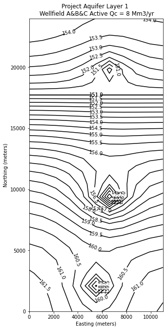
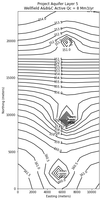
So for the stated problem, wellfield C is limited to about \(8~\frac{Mm^3}{yr}\) if the goal is to avoid river flow into the aquifer.
The next steps are to add stress periods according to the annual pumping schedule to examine the effect time-of-year has on the heads.
References
MODFLOW Notes (Cleveland circa 1992) The Obleo Aquifer simulation in the MODFLOW88 video is described in these notes.
MODFLOW Manual (US EPA) An EPA training document on the use of MODFLOW
