MODFLOW Program
Introduction
Adapted from https://pubs.usgs.gov/fs/FS-121-97/
The modular finite-difference groundwater flow model (MODFLOW) developed by the U.S. Geological Survey (USGS) is a computer program for simulating common features in groundwater systems (McDonald and Har- baugh, 1988; Harbaugh and McDonald, 1996). The program was constructed in the ear- ly 1980s and has continually evolved since then with development of many new packages and related programs for groundwater studies. Currently MODFLOW is the most widely used program in the world for simulating ground- water flow. The popularity of the program is attributed to the following factors:
The finite-difference method used by MODFLOW is relatively easy to understand and apply to a wide variety of real-world conditions.
MODDFLOW works on many different computer systems ranging from personal computers to super computers.
MODFLOW can be applied as a one- dimensional, two-dimensional, or quasi- or full three-dimensional model.
Each simulation feature of MODFLOW has been evensively tested.
Data input instructions and theory are well documented.
The modular program design of MODFLOW allows for new simulation features to be added with relative ease.
A wide variety of computer programs written by the USGS, other federal agencies, and private companies are available to analyze field data and con- struct input data sets for MODFLOW.
A wide variety of programs are available to read output from MODFLOW and graphically present model results in ways that are easily understood.
MODFLOW has been accepted in many court cases in the United States as a legitimate approach to analysis of groundwater systems.
Modeling
Modeling is a tool used by engineers to make decisions regarding design and operation of an environmental system. Models can be used to forecast future conditions in response to those decisions, select a best set of decisions based on some desired criterion, or determine the most likely physical values that explain an observed condition.
Because most real systems are far too complicated to model as they are, a set of simplifying assumptions is posed to make the modeling problem tractable - this is often called the “conceptual model”.
On the basis of these simplifying assumptions a “mathematical model” (usually balance equations) is created. The solution of the mathematical model yields the behavior of the system being studied.
After the model is created, it is “calibrated”. This is the process of adjusting model parameters (transmissivity, storativity, etc.), forcing inputs, and geometry until the model response is identical (within some tolerance) to the observed historical response of the real system. Multiple calibrations can produce identical responses, so great care must be taken in calibrating and testing a model before using it - once acceptably calibrated the model can be used for forecasting.
Classification of Environmental Models:
Physical models (experimentation) - usually impractical for groundwater ‘systems’.
Analog Models
Mathematical Models
Analytical solutions - application of calculus to achieve closed-form equations (some of which can be very difficult to evaluate).
Numerical solutions - application of numerical methods to achieve accurate approximations to the governing equations.
MODFLOW 6 (Using your own computer)
This would be the preferred way to use MODFLOW for this class. The install is not that hard, but alos not point and click. A video showing an installation is available for viewing at:
The installation process is:
GOOGLE “modflow 6” and/or select: https://www.usgs.gov/software/modflow-6-usgs-modular-hydrologic-model Download the MODFLOW 6 program (choose windows installer)
GOOGLE “ModelMuse” and/or select: https://www.usgs.gov/software/modelmuse-a-graphical-user-interface-groundwater-models Download the interface program (installer for 32/64 bit. Do not commit to 64 bit only (it might not work well). When you get a real job, have an IT professional do the install and testing)
Create C:/WRDAPP folder to house modflow binaries - note the folder attaches at C:/ any other path will probably mess things up later on.
Install ModelMuse using installer (double click, accept defaults)
Move the modflow package into C:/WRDAPP folder, extract package, put into folder root.
Start ModelMuse
create MODFLOW
next
next
Model/MODFLOW Program Locations
set the directory path (may need to edit names a bit)
Restart ModelMuse and run tutorial.
Pray for smiley faces!
Yay! Install complete.
MODFLOW 1988 (On-Line Structured Input Files)
A functioning web-accessible implementation of MODFLOW88 is available at 54.243.252.9. This is the hardest to use in terms of file management and error interpretation, but is reasonably easy to employ if using legacy files and the older documentation.
server name http://54.243.252.9/toolbox/gwhydraulics/modflow/
user name MODFLOW99
passwort On-Line
A video demonstrating the creation and running of a model using this implementation is available at YouTube.
MODFLOW Python Interfaces
A way to access MODFLOW using Python and Jupyter Notebooks is avaliable at
FloPy: Python Package for Creating, Running, and Post-Processing MODFLOW-Based Models
The PDF link below shows the installation and an example run on the AWS server.
Example from above link
# FloPy Example
import warnings
warnings.filterwarnings('ignore')

# arm/aarch need to compile mf6 on this chipset
# copy the result into a directory to house the scripts
# Run from JupyterBook -using absolute paths
# Seemed to run OK - now copy this into course notes and run from there
#
import os
import numpy as np
import matplotlib.pyplot as plt
import flopy
# Define grid
name = "example01_mf6"
h1 = 100
h2 = 90
Nlay = 10 #number layers
#Nrow = 101 #number rows
#Ncol = 101 #number columns
N = 101
L = 400.0 # length of sides
#Hx =
#Hy =
H = 50.0 # aquifer thickness
k = 1.0 # hydraulic condictivity

sim = flopy.mf6.MFSimulation(
    sim_name=name, exe_name="/home/sensei/ce-4363-webroot/ModflowExperimental/mf6-arm/mf6", version="mf6", sim_ws="/home/sensei/ce-4363-webroot/ModflowExperimental/mf6-arm/"
)
/opt/jupyterhub/lib/python3.8/site-packages/ipykernel/ipkernel.py:287: DeprecationWarning: `should_run_async` will not call `transform_cell` automatically in the future. Please pass the result to `transformed_cell` argument and any exception that happen during thetransform in `preprocessing_exc_tuple` in IPython 7.17 and above.
  and should_run_async(code)
tdis = flopy.mf6.ModflowTdis(
    sim, pname="tdis", time_units="DAYS", nper=1, perioddata=[(1.0, 1, 1.0)]
)
/opt/jupyterhub/lib/python3.8/site-packages/ipykernel/ipkernel.py:287: DeprecationWarning: `should_run_async` will not call `transform_cell` automatically in the future. Please pass the result to `transformed_cell` argument and any exception that happen during thetransform in `preprocessing_exc_tuple` in IPython 7.17 and above.
  and should_run_async(code)
ims = flopy.mf6.ModflowIms(sim, pname="ims", complexity="SIMPLE")
/opt/jupyterhub/lib/python3.8/site-packages/ipykernel/ipkernel.py:287: DeprecationWarning: `should_run_async` will not call `transform_cell` automatically in the future. Please pass the result to `transformed_cell` argument and any exception that happen during thetransform in `preprocessing_exc_tuple` in IPython 7.17 and above.
  and should_run_async(code)
model_nam_file = "{}.nam".format(name)
gwf = flopy.mf6.ModflowGwf(sim, modelname=name, model_nam_file=model_nam_file)
/opt/jupyterhub/lib/python3.8/site-packages/ipykernel/ipkernel.py:287: DeprecationWarning: `should_run_async` will not call `transform_cell` automatically in the future. Please pass the result to `transformed_cell` argument and any exception that happen during thetransform in `preprocessing_exc_tuple` in IPython 7.17 and above.
  and should_run_async(code)
bot = np.linspace(-H / Nlay, -H, Nlay)
delrow = delcol = L / (N - 1)
dis = flopy.mf6.ModflowGwfdis(
    gwf,
    nlay=Nlay,
    nrow=N,
    ncol=N,
    delr=delrow,
    delc=delcol,
    top=0.0,
    botm=bot,
)
/opt/jupyterhub/lib/python3.8/site-packages/ipykernel/ipkernel.py:287: DeprecationWarning: `should_run_async` will not call `transform_cell` automatically in the future. Please pass the result to `transformed_cell` argument and any exception that happen during thetransform in `preprocessing_exc_tuple` in IPython 7.17 and above.
  and should_run_async(code)
start = h1 * np.ones((Nlay, N, N))
ic = flopy.mf6.ModflowGwfic(gwf, pname="ic", strt=start)
/opt/jupyterhub/lib/python3.8/site-packages/ipykernel/ipkernel.py:287: DeprecationWarning: `should_run_async` will not call `transform_cell` automatically in the future. Please pass the result to `transformed_cell` argument and any exception that happen during thetransform in `preprocessing_exc_tuple` in IPython 7.17 and above.
  and should_run_async(code)
npf = flopy.mf6.ModflowGwfnpf(gwf, icelltype=1, k=k, save_flows=True)
/opt/jupyterhub/lib/python3.8/site-packages/ipykernel/ipkernel.py:287: DeprecationWarning: `should_run_async` will not call `transform_cell` automatically in the future. Please pass the result to `transformed_cell` argument and any exception that happen during thetransform in `preprocessing_exc_tuple` in IPython 7.17 and above.
  and should_run_async(code)
chd_rec = []
chd_rec.append(((0, int(N / 4), int(N / 4)), h2))
for layer in range(0, Nlay):
    for row_col in range(0, N):
        chd_rec.append(((layer, row_col, 0), h1))
        chd_rec.append(((layer, row_col, N - 1), h1))
        if row_col != 0 and row_col != N - 1:
            chd_rec.append(((layer, 0, row_col), h1))
            chd_rec.append(((layer, N - 1, row_col), h1))
chd = flopy.mf6.ModflowGwfchd(
    gwf,
    maxbound=len(chd_rec),
    stress_period_data=chd_rec,
    save_flows=True,
)
/opt/jupyterhub/lib/python3.8/site-packages/ipykernel/ipkernel.py:287: DeprecationWarning: `should_run_async` will not call `transform_cell` automatically in the future. Please pass the result to `transformed_cell` argument and any exception that happen during thetransform in `preprocessing_exc_tuple` in IPython 7.17 and above.
  and should_run_async(code)
iper = 0
ra = chd.stress_period_data.get_data(key=iper)
ra
/opt/jupyterhub/lib/python3.8/site-packages/ipykernel/ipkernel.py:287: DeprecationWarning: `should_run_async` will not call `transform_cell` automatically in the future. Please pass the result to `transformed_cell` argument and any exception that happen during thetransform in `preprocessing_exc_tuple` in IPython 7.17 and above.
  and should_run_async(code)
rec.array([((0, 25, 25),  90.), ((0, 0, 0), 100.), ((0, 0, 100), 100.),
           ..., ((9, 100, 99), 100.), ((9, 100, 0), 100.),
           ((9, 100, 100), 100.)],
          dtype=[('cellid', 'O'), ('head', '<f8')])
# Create the output control (`OC`) Package
headfile = "{}.hds".format(name)
head_filerecord = [headfile]
budgetfile = "{}.cbb".format(name)
budget_filerecord = [budgetfile]
saverecord = [("HEAD", "ALL"), ("BUDGET", "ALL")]
printrecord = [("HEAD", "LAST")]
oc = flopy.mf6.ModflowGwfoc(
    gwf,
    saverecord=saverecord,
    head_filerecord=head_filerecord,
    budget_filerecord=budget_filerecord,
    printrecord=printrecord,
)
/opt/jupyterhub/lib/python3.8/site-packages/ipykernel/ipkernel.py:287: DeprecationWarning: `should_run_async` will not call `transform_cell` automatically in the future. Please pass the result to `transformed_cell` argument and any exception that happen during thetransform in `preprocessing_exc_tuple` in IPython 7.17 and above.
  and should_run_async(code)
sim.write_simulation()
/opt/jupyterhub/lib/python3.8/site-packages/ipykernel/ipkernel.py:287: DeprecationWarning: `should_run_async` will not call `transform_cell` automatically in the future. Please pass the result to `transformed_cell` argument and any exception that happen during thetransform in `preprocessing_exc_tuple` in IPython 7.17 and above.
  and should_run_async(code)
writing simulation...
  writing simulation name file...
  writing simulation tdis package...
  writing ims package ims...
  writing model example01_mf6...
    writing model name file...
    writing package dis...
    writing package ic...
    writing package npf...
    writing package chd_0...
writing package oc...
success, buff = sim.run_simulation()
if not success:
    raise Exception("MODFLOW 6 did not terminate normally.")
FloPy is using the following executable to run the model: /home/sensei/ce-4363-webroot/ModflowExperimental/mf6-arm/mf6
                                   MODFLOW 6
                U.S. GEOLOGICAL SURVEY MODULAR HYDROLOGIC MODEL
                        VERSION 6.4.1 Release 12/09/2022

         MODFLOW 6 compiled Apr 16 2023 18:27:14 with GCC version 9.4.0

This software has been approved for release by the U.S. Geological
Survey (USGS). Although the software has been subjected to rigorous
review, the USGS reserves the right to update the software as needed
pursuant to further analysis and review. No warranty, expressed or
implied, is made by the USGS or the U.S. Government as to the
functionality of the software and related material nor shall the
fact of release constitute any such warranty. Furthermore, the
software is released on condition that neither the USGS nor the U.S.
Government shall be held liable for any damages resulting from its
authorized or unauthorized use. Also refer to the USGS Water
Resources Software User Rights Notice for complete use, copyright,
and distribution information.


 Run start date and time (yyyy/mm/dd hh:mm:ss): 2024/02/01 17:48:23

 Writing simulation list file: mfsim.lst
 Using Simulation name file: mfsim.nam
/opt/jupyterhub/lib/python3.8/site-packages/ipykernel/ipkernel.py:287: DeprecationWarning: `should_run_async` will not call `transform_cell` automatically in the future. Please pass the result to `transformed_cell` argument and any exception that happen during thetransform in `preprocessing_exc_tuple` in IPython 7.17 and above.
  and should_run_async(code)
Solving: Stress period: 1 Time step: 1
 Run end date and time (yyyy/mm/dd hh:mm:ss): 2024/02/01 17:48:25
 Elapsed run time:  1.934 Seconds

 Normal termination of simulation.
# now attempt to postprocess
h = gwf.output.head().get_data(kstpkper=(0, 0))
x = y = np.linspace(0, L, N)
y = y[::-1]
vmin, vmax = 90.0, 100.0
contour_intervals = np.arange(90, 100.1, 1.0)
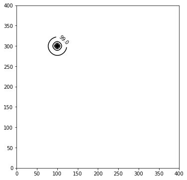
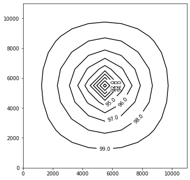
# ### Plot a Map of Layer 1
fig = plt.figure(figsize=(6, 6))
ax = fig.add_subplot(1, 1, 1, aspect="equal")
c = ax.contour(x, y, h[0], contour_intervals, colors="black")
plt.clabel(c, fmt="%2.1f")
/opt/jupyterhub/lib/python3.8/site-packages/ipykernel/ipkernel.py:287: DeprecationWarning: `should_run_async` will not call `transform_cell` automatically in the future. Please pass the result to `transformed_cell` argument and any exception that happen during thetransform in `preprocessing_exc_tuple` in IPython 7.17 and above.
  and should_run_async(code)
<a list of 1 text.Text objects>
# ### Plot a Map of Layer 10

x = y = np.linspace(0, L, N)
y = y[::-1]
fig = plt.figure(figsize=(6, 6))
ax = fig.add_subplot(1, 1, 1, aspect="equal")
c = ax.contour(x, y, h[-1], contour_intervals, colors="black")
plt.clabel(c, fmt="%1.1f")
/opt/jupyterhub/lib/python3.8/site-packages/ipykernel/ipkernel.py:287: DeprecationWarning: `should_run_async` will not call `transform_cell` automatically in the future. Please pass the result to `transformed_cell` argument and any exception that happen during thetransform in `preprocessing_exc_tuple` in IPython 7.17 and above.
  and should_run_async(code)
<a list of 0 text.Text objects>
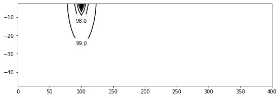
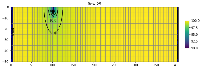
# ### Plot a Cross-section along row 25

z = np.linspace(-H / Nlay / 2, -H + H / Nlay / 2, Nlay)
fig = plt.figure(figsize=(9, 3))
ax = fig.add_subplot(1, 1, 1, aspect="auto")
c = ax.contour(x, z, h[:, int(N / 4), :], contour_intervals, colors="black")
plt.clabel(c, fmt="%1.1f")
/opt/jupyterhub/lib/python3.8/site-packages/ipykernel/ipkernel.py:287: DeprecationWarning: `should_run_async` will not call `transform_cell` automatically in the future. Please pass the result to `transformed_cell` argument and any exception that happen during thetransform in `preprocessing_exc_tuple` in IPython 7.17 and above.
  and should_run_async(code)
<a list of 2 text.Text objects>
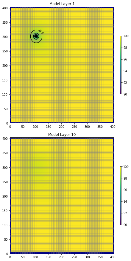
# ### Use the FloPy `PlotMapView()` capabilities for MODFLOW 6
#
# ### Plot a Map of heads in Layers 1 and 10

fig, axes = plt.subplots(2, 1, figsize=(6, 12), constrained_layout=True)
# first subplot
ax = axes[0]
ax.set_title("Model Layer 1")
modelmap = flopy.plot.PlotMapView(model=gwf, ax=ax)
pa = modelmap.plot_array(h, vmin=vmin, vmax=vmax)
quadmesh = modelmap.plot_bc("CHD")
linecollection = modelmap.plot_grid(lw=0.5, color="0.5")
contours = modelmap.contour_array(
    h,
    levels=contour_intervals,
    colors="black",
)
ax.clabel(contours, fmt="%2.1f")
cb = plt.colorbar(pa, shrink=0.5, ax=ax)
# second subplot
ax = axes[1]
ax.set_title(f"Model Layer {Nlay}")
modelmap = flopy.plot.PlotMapView(model=gwf, ax=ax, layer=Nlay - 1)
linecollection = modelmap.plot_grid(lw=0.5, color="0.5")
pa = modelmap.plot_array(h, vmin=vmin, vmax=vmax)
quadmesh = modelmap.plot_bc("CHD")
contours = modelmap.contour_array(
    h,
    levels=contour_intervals,
    colors="black",
)
ax.clabel(contours, fmt="%2.1f")
cb = plt.colorbar(pa, shrink=0.5, ax=ax)
/opt/jupyterhub/lib/python3.8/site-packages/ipykernel/ipkernel.py:287: DeprecationWarning: `should_run_async` will not call `transform_cell` automatically in the future. Please pass the result to `transformed_cell` argument and any exception that happen during thetransform in `preprocessing_exc_tuple` in IPython 7.17 and above.
  and should_run_async(code)
# ### Use the FloPy `PlotCrossSection()` capabilities for MODFLOW 6
#
# ### Plot a cross-section of heads along row 25

fig, ax = plt.subplots(1, 1, figsize=(9, 3), constrained_layout=True)
# first subplot
ax.set_title("Row 25")
modelmap = flopy.plot.PlotCrossSection(
    model=gwf,
    ax=ax,
    line={"row": int(N / 4)},
)
pa = modelmap.plot_array(h, vmin=vmin, vmax=vmax)
quadmesh = modelmap.plot_bc("CHD")
linecollection = modelmap.plot_grid(lw=0.5, color="0.5")
contours = modelmap.contour_array(
    h,
    levels=contour_intervals,
    colors="black",
)
ax.clabel(contours, fmt="%2.1f")
cb = plt.colorbar(pa, shrink=0.5, ax=ax)
/opt/jupyterhub/lib/python3.8/site-packages/ipykernel/ipkernel.py:287: DeprecationWarning: `should_run_async` will not call `transform_cell` automatically in the future. Please pass the result to `transformed_cell` argument and any exception that happen during thetransform in `preprocessing_exc_tuple` in IPython 7.17 and above.
  and should_run_async(code)
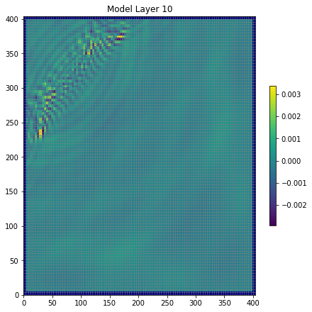
# ## Determine the Flow Residual
#
# The `FLOW-JA-FACE` cell-by-cell budget data can be processed to
# determine the flow residual for each cell in a MODFLOW 6 model. The
# diagonal position for each row in the `FLOW-JA-FACE` cell-by-cell
# budget data contains the flow residual for each cell and can be
# extracted using the `flopy.mf6.utils.get_residuals()` function.
#
# First extract the `FLOW-JA-FACE` array from the cell-by-cell budget file

flowja = gwf.oc.output.budget().get_data(text="FLOW-JA-FACE", kstpkper=(0, 0))[
    0
]

# Next extract the flow residual. The MODFLOW 6 binary grid file is passed
# into the function because it contains the ia array that defines
# the location of the diagonal position in the `FLOW-JA-FACE` array.

grb_file = "/home/sensei/ce-4363-webroot/ModflowExperimental/mf6-arm/" + f"{name}.dis.grb"
#grb_file = workspace + ".dis.grb"
residual = flopy.mf6.utils.get_residuals(flowja, grb_file=grb_file)

# ### Plot a Map of the flow error in Layer 10

fig, ax = plt.subplots(1, 1, figsize=(6, 6), constrained_layout=True)
ax.set_title("Model Layer 10")
modelmap = flopy.plot.PlotMapView(model=gwf, ax=ax, layer=Nlay - 1)
pa = modelmap.plot_array(residual)
quadmesh = modelmap.plot_bc("CHD")
linecollection = modelmap.plot_grid(lw=0.5, color="0.5")
contours = modelmap.contour_array(
    h,
    levels=contour_intervals,
    colors="black",
)
ax.clabel(contours, fmt="%2.1f")
plt.colorbar(pa, shrink=0.5)
/opt/jupyterhub/lib/python3.8/site-packages/ipykernel/ipkernel.py:287: DeprecationWarning: `should_run_async` will not call `transform_cell` automatically in the future. Please pass the result to `transformed_cell` argument and any exception that happen during thetransform in `preprocessing_exc_tuple` in IPython 7.17 and above.
  and should_run_async(code)
<matplotlib.colorbar.Colorbar at 0xffff8132cb50>
Series of Examples
Example 1
This example is a single well
import warnings
warnings.filterwarnings('ignore')
import os
import numpy as np
import matplotlib.pyplot as plt
import flopy
/opt/jupyterhub/lib/python3.8/site-packages/ipykernel/ipkernel.py:287: DeprecationWarning: `should_run_async` will not call `transform_cell` automatically in the future. Please pass the result to `transformed_cell` argument and any exception that happen during thetransform in `preprocessing_exc_tuple` in IPython 7.17 and above.
  and should_run_async(code)
# Workspace and Executibles
binary = "/home/sensei/ce-4363-webroot/ModflowExperimental/mf6-arm/mf6"  # location on MY computer of the compiled modflow program
workarea = "/home/sensei/ce-4363-webroot/ModflowExperimental/mf6-arm/example_1" # location on MY computer to store files this example (directory must already exist)

# Set Simulation Name
name = "example01_obleo"

##### FLOPY Build simulation framework ####
sim = flopy.mf6.MFSimulation(
    sim_name=name, exe_name=binary, version="mf6", sim_ws=workarea
)
# Set Time Structure
Time_Units="DAYS"

##### FLOPY Build time framework ##########
tdis = flopy.mf6.ModflowTdis(
    sim, pname="tdis", time_units=Time_Units, nper=1, perioddata=[(1.0, 1, 1.0)]
)
# Set Iterative Model Solution (choose solver parameters)
# about IMS see: https://water.usgs.gov/nrp/gwsoftware/ModelMuse/Help/sms_sparse_matrix_solution_pac.htm
# using defaults see: https://flopy.readthedocs.io/en/3.3.2/source/flopy.mf6.modflow.mfims.html

##### FLOPY Build IMS framework ###########
ims = flopy.mf6.ModflowIms(sim, pname="ims", complexity="SIMPLE")
# Set Model Name (using same base name as the simulation)
model_nam_file = "{}.nam".format(name)

##### FLOPY Build Model Name framework ####
gwf = flopy.mf6.ModflowGwf(sim, modelname=name, model_nam_file=model_nam_file)
# Define The Grid
Nlay = 1 #number layers
Nrow = 11 #number rows
Ncol = 11 #number columns
# Define distances and elevations
delrow = 1000 # cell size along columns (how tall is a row)
delcol = 1000 # cell size along row (how wide is a column)
top = 0.0 # elevation of top of model
thick = 50.0 #aquifer thickness

bot = np.linspace(-thick / Nlay, -thick, Nlay)


##### FLOPY Build Model Grid framework #####
dis = flopy.mf6.ModflowGwfdis(gwf,nlay=Nlay,nrow=Nrow,ncol=Ncol,delr=delrow,delc=delcol,top=0.0,botm=bot,
)
# Define initial conditions
h1 = 100.0 #
start = h1 * np.ones((Nlay, Nrow, Ncol)) # start heads are h1 everywhere

##### FLOPY Build Initial Conditions framework ###
ic = flopy.mf6.ModflowGwfic(gwf, pname="ic", strt=start)
# Define hydraulic conductivity arrays
K = 1.0
k = K * np.ones((Nlay, Nrow, Ncol)) # Hydraulic conductivity is K everywhere
# Use above to build layer-by-layer spatial varying K
# need to read: to deal with Kx!=Ky


##### FLOPY Build BCF framework ######
npf = flopy.mf6.ModflowGwfnpf(gwf, icelltype=1, k=k, save_flows=True)
# Define constant head boundary conditions
chd_rec = []
#h2 = 90 # Just a different value
#chd_rec.append(((0, 5, 5), h2))
# L,R,T,B constant head boundaries
for layer in range(0, Nlay):
    for row in range(0, Nrow):
        chd_rec.append(((layer, row, 0), h1))  #left column held at h1
        chd_rec.append(((layer, row, Ncol-1), h1)) #right column held at h1
    for col in range(1,Ncol-1):
        chd_rec.append(((layer, 0, col), h1)) #top row held at h1
        chd_rec.append(((layer, Nrow-1 , col), h1))


##### FLOPY Build CHD framework #####
chd = flopy.mf6.ModflowGwfchd(gwf,maxbound=len(chd_rec),stress_period_data=chd_rec,save_flows=True,
)
# Define wellfields
wel_rec = []
wel_rec.append((0, 5, 5, -1000)) #

##### FLOPY Build Wellfields framework #####
wel = flopy.mf6.ModflowGwfwel(gwf,maxbound=len(wel_rec),stress_period_data=wel_rec,
)
# something to do with stress periods
iper = 0
ra = chd.stress_period_data.get_data(key=iper)
# Create the output control (`OC`) Package
headfile = "{}.hds".format(name)
head_filerecord = [headfile]
budgetfile = "{}.cbb".format(name)
budget_filerecord = [budgetfile]
saverecord = [("HEAD", "ALL"), ("BUDGET", "ALL")]
printrecord = [("HEAD", "LAST")]

##### FLOPY Build OC framework
oc = flopy.mf6.ModflowGwfoc(
    gwf,
    saverecord=saverecord,
    head_filerecord=head_filerecord,
    budget_filerecord=budget_filerecord,
    printrecord=printrecord,
)
# Write files to the directory
sim.write_simulation()
writing simulation...
  writing simulation name file...
  writing simulation tdis package...
  writing ims package ims...
  writing model example01_obleo...
    writing model name file...
    writing package dis...
    writing package ic...
    writing package npf...
    writing package chd_0...
    writing package wel_0...
    writing package oc...
# Attempt to run MODFLOW this model
success, buff = sim.run_simulation()
if not success:
    raise Exception("MODFLOW 6 did not terminate normally.")
FloPy is using the following executable to run the model: /home/sensei/ce-4363-webroot/ModflowExperimental/mf6-arm/mf6
                                   MODFLOW 6
                U.S. GEOLOGICAL SURVEY MODULAR HYDROLOGIC MODEL
                        VERSION 6.4.1 Release 12/09/2022

         MODFLOW 6 compiled Apr 16 2023 18:27:14 with GCC version 9.4.0

This software has been approved for release by the U.S. Geological
Survey (USGS). Although the software has been subjected to rigorous
review, the USGS reserves the right to update the software as needed
pursuant to further analysis and review. No warranty, expressed or
implied, is made by the USGS or the U.S. Government as to the
functionality of the software and related material nor shall the
fact of release constitute any such warranty. Furthermore, the
software is released on condition that neither the USGS nor the U.S.
Government shall be held liable for any damages resulting from its
authorized or unauthorized use. Also refer to the USGS Water
Resources Software User Rights Notice for complete use, copyright,
and distribution information.


 Run start date and time (yyyy/mm/dd hh:mm:ss): 2024/02/01 17:48:34

 Writing simulation list file: mfsim.lst
 Using Simulation name file: mfsim.nam

    Solving:  Stress period:     1    Time step:     1

 Run end date and time (yyyy/mm/dd hh:mm:ss): 2024/02/01 17:48:34
 Elapsed run time:  0.026 Seconds

 Normal termination of simulation.
# now attempt to postprocess
h = gwf.output.head().get_data(kstpkper=(0, 0))
x =  np.linspace(0, delrow*Ncol, Ncol)
y =  np.linspace(0, delrow*Nrow, Nrow)
y = y[::-1]
vmin, vmax = -0, 110.0
contour_intervals = np.arange(-0., 110., 1.0)

# ### Plot a Map of Layer 1

fig = plt.figure(figsize=(6, 6))
ax = fig.add_subplot(1, 1, 1, aspect="equal")
c = ax.contour(x, y, h[0], contour_intervals, colors="black")
plt.clabel(c, fmt="%2.1f")
<a list of 8 text.Text objects>
# second subplot
ax = axes[1]
ax.set_title(f"Model Layer {Nlay}")
modelmap = flopy.plot.PlotMapView(model=gwf, ax=ax, layer=Nlay - 1)
linecollection = modelmap.plot_grid(lw=0.5, color="0.5")
pa = modelmap.plot_array(h, vmin=vmin, vmax=vmax)
quadmesh = modelmap.plot_bc("CHD")
contours = modelmap.contour_array(
    h,
    levels=contour_intervals,
    colors="black",
)
ax.clabel(contours, fmt="%2.1f")
cb = plt.colorbar(pa, shrink=0.5, ax=ax)
References
MODFLOW Notes (Cleveland circa 1992) The Obleo Aquifer simulation in the MODFLOW88 video is described in these notes.
MODFLOW Manual (US EPA) An EPA training document on the use of MODFLOW