Groundwater Flow to Wells - II (pp. 162 - 166)
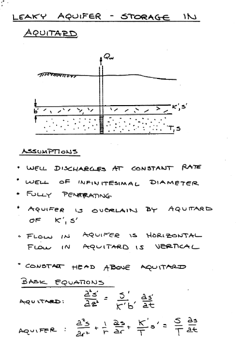
Leaky Confining Layer (No storage in the confining layer) A.K.A. Hantush (1956) Solution
Situation Set-Up and Mathematical Considerations
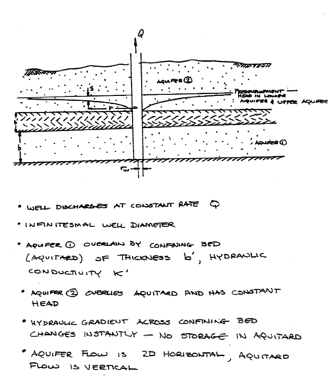
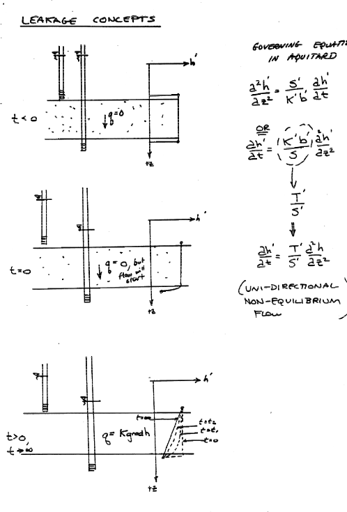
Leakance Considerations
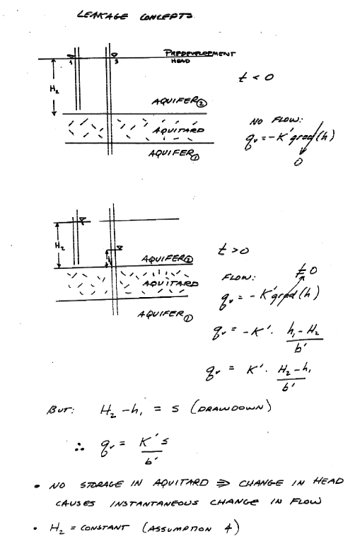
Mathematical Model
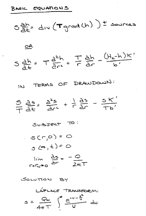
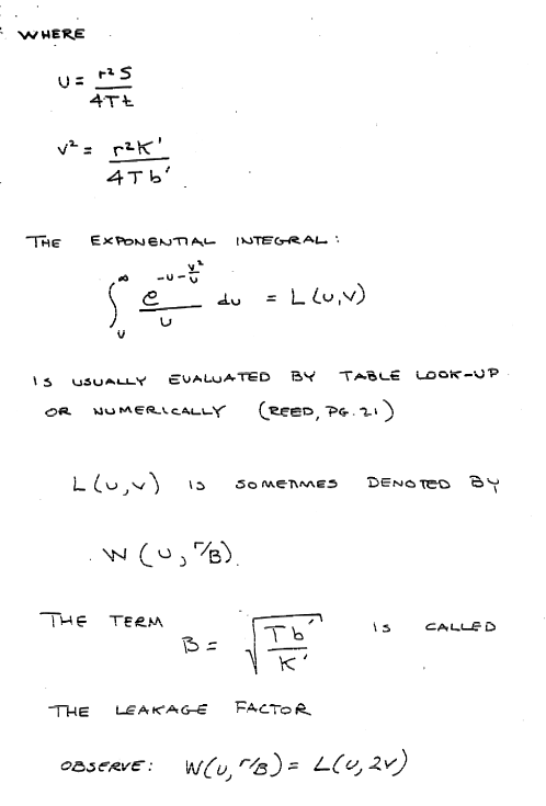
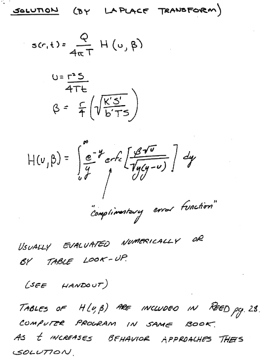
Solutions
def wh(u, rho): # Hantush Leaky aquifer well function
    import numpy
    """Returns Hantush's well function values

    Note: works only for scalar values of u and rho

    Parameters:
    -----------
    u : scalar  (u= r^2 * S / (4 * kD * t))
    rho : sclaar (rho =r / lambda, lambda = sqrt(kD * c))
    Returns:
    --------
    Wh(u, rho) : Hantush well function value for (u, rho)
    """
    try:
        u =float(u)
        rho =float(rho)
    except:
        print("u and rho must be scalars.")
        raise ValueError()

    LOGINF = 2
    y = numpy.logspace(numpy.log10(u), LOGINF, 1000)
    ym = 0.5 * (y[:-1]+  y[1:])
    dy = numpy.diff(y)
    wh = numpy.sum(numpy.exp(-ym - (rho / 2)**2 / ym ) * dy / ym)
    return wh

wh(0.625,5)
0.007379841673127564
Example on pg. 165 to illustrate homebrew script
The relevant problem parametrs are:
\(K = 0.73 m/d\)
\(b = 5.2 m\)
\(T = Kb = 3.8 m^2/d\)
\(S = 0.0035\)
\(Q_w = 28 m^3/d\)
\(b' = 1.1 m\)
\(K'_v = 5.5 \times 10^{-5} m/d\)
Notice in the example the author tests some requesite assumptions before proceeding to look up values in a table (also a good idea here, but we will just be lazy and apply the script)
def leaky(radius,time,storage,transmissivity,discharge,leakance): # Leaky drawdown function using Hantush solution
    import math
    u = ((radius**2)*(storage))/(4*transmissivity*time)
    roB = radius/leakance
    leaky = ((discharge)/(4*math.pi*transmissivity))*wh(u,roB)
    return(leaky)
import math
radius=[1.5,5.5,10,25,75,150]
ddn=[0 for i in range(len(radius))] # list of zeros to hold results
# simulation constants
time = 1 # 1 day
transmissivity = 3.8
storage = 0.0035
discharge = 28
bprime = 1.1
Kvert = 5.5e-05
# computed constants
B = math.sqrt((transmissivity*bprime)/Kvert)
# compute the drawdowns
for i in range(len(radius)):
    ddn[i]=leaky(radius[i],time,storage,transmissivity,discharge,B)
# print results
print("radius    drawdown   ")
for i in range(len(radius)):
    print(round(radius[i],1),round(ddn[i],3))
radius    drawdown
1.5 4.089
5.5 2.57
10 1.879
25 0.874
75 0.079
150 0.001
Leaky Confining Layer (No storage in the confining layer)
Situation Set-Up and Mathematical Considerations
Leakance Considerations
Mathematical Model
Solutions
Usually solutions are approximated for early-time, mid-time, and late-time behavior and use combinations of Theis solutions and finite-term series. The actual integral can certainly be evaluated if needed, but modern (circa-2023) approaches would probably be to finite-difference the crap out of things and take the numerical solution as good enough!