3. Fundamentals (Practice)

3. Fundamentals (Practice)#

Course Website

%%html
<style> table {margin-left: 0 !important;} </style>

import sys, subprocess
hostname = subprocess.check_output("hostname", shell=True, text=True).strip(); username = subprocess.check_output("whoami", shell=True, text=True).strip()
python_executable = sys.executable; python_version = sys.version; python_version_info = sys.version_info
print(f"Hostname: {hostname}\n" f"User: {username}\n" f"Python Executable: {python_executable}\n" f"Python Version: {python_version}\n" f"Python Version Info: {python_version_info}")

Hostname: ip-172-26-5-168
User: sensei
Python Executable: /opt/jupyterhub/bin/python3
Python Version: 3.10.12 (main, May 27 2025, 17:12:29) [GCC 11.4.0]
Python Version Info: sys.version_info(major=3, minor=10, micro=12, releaselevel='final', serial=0)

Scope#

flow equations
transport equations
generating flow nets (practical)

Readings#

Videos#

None

Spreadsheets/Programs/Data#

None

Flow Equations#

The governing equations for groundwater flow are derived by combining Darcy’s law—which describes how water moves through porous media under a hydraulic gradient—with the principle of mass conservation applied to a representative elementary volume (REV) of the aquifer. The result is a partial differential equation that relates changes in hydraulic head over time to the spatial variation in flow and any external sources or sinks of water. The specific form of the equation depends on the aquifer type, dimensionality, and storage properties.

Unconfined Aquifer:

For an unconfined aquifer, the saturated thickness of the aquifer changes as water levels rise and fall. In this case, transmissivity depends on the instantaneous head, so the conductivity terms are multiplied by $h$. The left-hand side contains the product of the specific yield $S_y$ and the rate of change of head $\frac{\partial h}{\partial t}$, reflecting the volume of water released from storage per unit surface area per unit decline in head. The right-hand side sums the divergence of the flow in the $x$ and $y$ directions, and adds (or subtracts) source/sink terms for recharge, pumping, or leakage.

\[S_y \frac{\partial h}{\partial t} = \frac{\partial}{\partial x}(K_x h \frac{\partial h}{\partial x}) + \frac{\partial}{\partial y}(K_y h \frac{\partial h}{\partial y}) \pm source/sink \]

where:

$S_y$ = specific yield.

Confined Aquifer (3D) :

In a confined aquifer, the saturated thickness remains constant, so transmissivity is independent of head. Instead, storage comes from the compressibility of the aquifer matrix and the pore water, represented in the specific storage term $S_s =\rho g (\alpha + n \beta)$, where $\alpha$ is the matrix compressibility, $\beta$ is the fluid compressibility, $n$ is porosity, $\rho$ is fluid density, and $g$ is gravitational acceleration. The fully three-dimensional form accounts for anisotropic conductivities $K_x,K_y,K_z$ in all directions.

\[S_s \frac{\partial h}{\partial t} = \frac{\partial}{\partial x}(K_x\frac{\partial h}{\partial x}) + \frac{\partial}{\partial y}(K_y\frac{\partial h}{\partial y}) + \frac{\partial}{\partial z}(K_z\frac{\partial h}{\partial z})\pm source/sink \]

where:

$S_s =\rho g (\alpha + n \beta)$.
$\alpha$ = compressibility of porous matrix (a spring constant for the solids fraction).
$\beta$ = compressibility of liquid (usually water).

Confined Aquifer (2D) :

When a confined aquifer can be treated in two dimensions—for example, in a horizontal flow model—the governing equation is vertically integrated over the aquifer thickness. The result is an equation in terms of transmissivity $T$ and storage coefficient $S$, where $S$ is the vertical integral of $S_s$ across the aquifer thickness. This 2D form is common in regional groundwater modeling where vertical gradients are small compared to horizontal gradients, and it simplifies computations while preserving the essential physics of lateral groundwater movement. A common extension is layers of 2D models with leakage between layers (quasi-3D).

\[S \frac{\partial h}{\partial t} = \frac{\partial}{\partial x}(T_x\frac{\partial h}{\partial x}) + \frac{\partial}{\partial y}(T_y\frac{\partial h}{\partial y}) \pm source/sink \]

where:

$S$ = storage coefficient ($S = \int_{z_{bot}}^{z_{top}}S_s(z) dz$

Note

Origin of these equations

Starting Point : Darcy’s law + conservation of mass

Darcy’s law (vector form, possibly anisotropic):

$𝑞=−𝐾 \nabla h$

where

$q$ is specific discharge
$K$ is the hydraulic conductivity tensor
h is hydraulic head (a scalar field)

Continuity (single-phase water, small deformations):

$\frac{\partial(\rho \theta)}{\partial t} + \nabla \cdot (\rho q) = \rho W$

$\theta$ is volumetric water content ($\approx~$ porosity $n$ when saturated), $W$ is a volumetric source/sink per bulk volume (positive = recharge), and $ρ$ is water density.

Assuming constant density (negligible variable-density effects) and rearranging:

$\frac{\partial \theta}{\partial t} + \nabla \cdot q = W$

All the physics now lives in (i) how $\theta$ changes with $h$ (storage) and (ii) $q$ from Darcy’s law.

Confined aquifer (3D)

In a confined aquifer, the saturated thickness is constant; storage arises from compressibility of the matrix and water. A decline $dh$ produces a volumetric water release $(S_s dh)$ per unit bulk volume, where

$S_s =\rho g (\alpha + n \beta)$

Here $\alpha$ is matrix compressibility, $\beta$ is water compressibility $n$ is porosity, $ρg$ converts head to pressure.

Thus

$\frac{\partial \theta}{\partial t}~\approx~S_s\frac{\partial h}{\partial t}$

Insert Darcy’s law $𝑞=−𝐾 \nabla h$ as the equation of motion into continuity:

$S_s\frac{\partial h}{\partial t}+ \nabla \cdot (−K \nabla h) = W \to S_s\frac{\partial h}{\partial t}= \nabla \cdot (K \nabla h) + W$

which in components gives the 3D confined equation:

$S_s \frac{\partial h}{\partial t} = \frac{\partial}{\partial x}(K_x\frac{\partial h}{\partial x})

\frac{\partial}{\partial y}(K_y\frac{\partial h}{\partial y}) + \frac{\partial}{\partial z}(K_z\frac{\partial h}{\partial z})\pm W (source/sink) $

Confined aquifer, vertically integrated (2D)

Integrate the 3D equation from $z_{bot}$ to $z_{top}$ (aquifer thickness $B$. Define:

$T_x = \int_{z_{bot}}^{z_{top}} K_x(z) dz~(\approx~K_xB)~~~~$ $T_y = \int_{z_{bot}}^{z_{top}} K_y(z) dz~(\approx~K_yB)~~~~$ $S = \int_{z_{bot}}^{z_{top}} S_s(z) dz~(\approx~S_sB)$

Assuming $h$ is nearly uniform with depth (Dupuit-type vertical averaging for confined systems), the vertical terms cancel on integration and sources/sinks convert to areal rates $W'$. The result is:

$S \frac{\partial h}{\partial t} = \frac{\partial}{\partial x}(T_x\frac{\partial h}{\partial x})

\frac{\partial}{\partial y}(T_y\frac{\partial h}{\partial y}) \pm W’ (source/sink) $

which is the 2D confined equation.

Unconfined aquifer (Boussinesq form)

For unconfined conditions, the saturated thickness equals the head above the impermeable base (take datum $z_b$) so the thickness is $b=h−z_b~\approx h ~\text{if}~z_b=0$. Two key changes:

Storage: draining/filling is dominated by specific yield $S_y$ (drainable porosity), so

$\frac{\partial \theta}{\partial t}~\approx~S_y \frac{\partial h}{\partial t}$.

Transmissivity depends on head: thickness $b \simeq h$, so the horizontal fluxes use head-dependent transmissivity:

$q_x=-K_x h \frac{\partial h}{\partial x}~~~~$,$q_y=-K_y h \frac{\partial h}{\partial y}~~~~$,

after invoking a Dupuit assumption (vertical gradients small compared to horizontal; vertical head distribution is nearly hydrostatic).

Insert into continuity (plan-view):

$S_y \frac{\partial h}{\partial t} = \frac{\partial}{\partial x}(K_x h \frac{\partial h}{\partial x})

\frac{\partial}{\partial y}(K_y h \frac{\partial h}{\partial y}) \pm W’ (source/sink) $

which is the Boussinesq equation used for unconfined flow (the equation above, with optional sources/sinks).

Transport Equations#

Transport builds on the same foundations as flow: the equations of motion (Darcy’s law) and mass continuity. Here we add constituent-specific processes—advection and hydrodynamic dispersion—plus reactions (e.g., decay, biodegradation) and sorption. Although sorption is a reaction, it’s often treated separately because it directly alters storage via retardation.

We assume a saturated medium with constant fluid density and porosity over the time scales of interest. The velocity field is obtained from the groundwater flow solution described above (using $\mathbf{q}$ or $\mathbf{v}=\mathbf{q}/n$ as appropriate).

Variables and constitutive pieces#

$C(\mathbf{x},t)$ — dissolved concentration $[M\,L^{-3}]$ in the mobile (water) phase
$s(\mathbf{x},t)$ — sorbed concentration on the solid phase $[M\,M^{-1}]$
$n$ — porosity $[-]$; $\ \rho_b$ — bulk density of porous medium $[M\,L^{-3}]$
$\mathbf{q}$ — Darcy flux (specific discharge) $[L\,T^{-1}]$
$\mathbf{v}=\mathbf{q}/n$ — average linear (pore) velocity $[L\,T^{-1}]$
$\boldsymbol{D}$ — hydrodynamic dispersion tensor $[L^{2}\,T^{-1}]$: $$ \boldsymbol{D} \;=\; \tau D_m\,\mathbf{I} \;+\; \alpha_T\,\lVert\mathbf{v}\rVert\,\mathbf{I} \;+\; (\alpha_L-\alpha_T)\,\frac{\mathbf{v}\mathbf{v}^{\!\top}}{\lVert\mathbf{v}\rVert} $$ where $D_m$ is molecular diffusion, $\tau$ is tortuosity, and $\alpha_L,\alpha_T$ are longitudinal/transverse dispersivities.
$W(\mathbf{x},t)$ — volumetric water source/sink per bulk volume $[T^{-1}]$ (positive = water addition)
$C_{\mathrm{in}}(\mathbf{x},t)$ — concentration of water added through $W>0$

Dissolved mass flux (dispersion + advection): $$ \mathbf{J} \;=\; -\,n\,\boldsymbol{D}\,\nabla C \;+\; \mathbf{q}\,C \qquad [M\,L^{-2}\,T^{-1}]. $$

Species mass balance over a representative elementary volume (REV)#

Total species mass per bulk volume: $$ M \;=\; nC \;+\; \rho_b s. $$

Conservation of mass (accumulation = inflow $-$ outflow $+$ reactions $+$ external additions): $$ \frac{\partial}{\partial t}\big(nC + \rho_b s\big) \;+\; \nabla\!\cdot\mathbf{J} \;=\; nW\,C_{\mathrm{in}} \;+\; R_{\text{chem}}(C,s,\ldots), $$ where $R_{\text{chem}}[M,L^{-3},T^{-1}]$ is net internal production/consumption from reactions not otherwise represented (e.g., multispecies kinetics, biodegradation).

Insert $\mathbf{J}$: $$ \frac{\partial}{\partial t}\big(nC + \rho_b s\big) \;+\; \nabla\!\cdot\!\big(-\,n\boldsymbol{D}\nabla C + \mathbf{q}C\big) \;=\; nW\,C_{\mathrm{in}} \;+\; R_{\text{chem}}. $$

Using groundwater continuity, $\nabla\!\cdot\mathbf{q}=nW$, we have
$-\nabla\!\cdot(\mathbf{q}C)= -\mathbf{q}\!\cdot\nabla C \;-\; C\,\nabla\!\cdot\mathbf{q} = -\mathbf{q}\!\cdot\nabla C - nW\,C$.
Together with $+\,nW\,C_{\mathrm{in}}$, the net water exchange term is $nW(C_{\mathrm{in}}-C)$.

Sorption and retardation (a type of reaction)#

(a) Instantaneous linear equilibrium sorption#

Assume $s = K_d\,C$. Then $$ \frac{\partial}{\partial t}(nC + \rho_b s) = \big(n + \rho_b K_d\big)\,\frac{\partial C}{\partial t} = n\,R_f\,\frac{\partial C}{\partial t}, \qquad R_f \equiv 1 + \frac{\rho_b K_d}{n}. $$

Substitute into the balance equation above:

\[nR_f \frac{\partial C}{\partial t} = \nabla\!\cdot\!\big(n\boldsymbol{D}\nabla C\big) - \nabla \cdot(\mathbf{q}C) + nW C_{\mathrm{in}} + R_{\text{chem}}(C) - \lambda n C,\]

where $-\lambda n C$ represents first-order aqueous decay (optional).

Divide by $n$ and use $\mathbf{v}=\mathbf{q}/n$ if preferred:

\[ R_f\,\frac{\partial C}{\partial t} = \nabla\!\cdot\!\big(\boldsymbol{D}\nabla C\big) - \nabla\!\cdot(\mathbf{v}C) + W\,C_{\mathrm{in}} + \frac{R_{\text{chem}}}{n} - \lambda\ C. \]

(b) Kinetic sorption (first-order two-rate; optional)#

Replace $s=K_d C$ with $$ \rho_b\frac{\partial s}{\partial t} = k_a\,\rho_b C \;-\; k_d\,\rho_b s, $$ and keep $\rho_b ,\partial s/\partial t$ explicitly in the accumulation term. No single $R_f$ applies; this yields a coupled PDE–ODE system.

(c) Dual-porosity / mobile–immobile (optional)#

Let $n = n_m + n_{im}$ and introduce $C_{im}$: $$ \begin{aligned} & n_m\frac{\partial C}{\partial t} + \rho_b\frac{\partial s}{\partial t} \;-\; \nabla\!\cdot\!\big(n_m\boldsymbol{D}\nabla C\big) + \nabla\!\cdot(\mathbf{q}C) = nW\,C_{\mathrm{in}} + R_{\text{chem}} - \omega\,(C_{im}-C) - \lambda\,n_m C, \\[4pt] & n_{im}\frac{\partial C_{im}}{\partial t} = \omega\,(C_{im}-C) - \lambda_{im}\,n_{im} C_{im}. \end{aligned} $$

Canonical forms (for direct use)#

General conservative form (no assumption on sorption kinetics): $$ \frac{\partial}{\partial t}\big(nC + \rho_b s\big) = \nabla\!\cdot\!\big(n\boldsymbol{D}\nabla C\big) - \nabla\!\cdot(\mathbf{q}C) + nW\,C_{\mathrm{in}} + R_{\text{chem}}(C,s,\ldots) - \lambda\,nC. $$

Retarded ADE with first-order decay (instantaneous linear sorption): $$ nR_f\,\frac{\partial C}{\partial t} = \nabla\!\cdot\!\big(n\boldsymbol{D}\nabla C\big) - \nabla\!\cdot(\mathbf{q}C) + nW\,C_{\mathrm{in}} + R_{\text{chem}}(C) - \lambda\,nC. $$

(Optionally divide by $n$ and write in terms of $\mathbf{v}=\mathbf{q}/n$.)

Boundary conditions (quick reference)#

Dirichlet (specified concentration): $C = C_b$ on $\Gamma_D$.
Neumann (specified mass flux): $\mathbf{n}\!\cdot\!\big(-n\boldsymbol{D}\nabla C + \mathbf{q}C\big) = J_b$ on $\Gamma_N$.
No-flux: $\mathbf{n}\!\cdot\!\big(-n\boldsymbol{D}\nabla C + \mathbf{q}C\big)=0$.

Units and sign checks#

$\nabla\!\cdot(n\boldsymbol{D}\nabla C)$ and $-\nabla\!\cdot(\mathbf{q}C)$ both have units $[M\,L^{-3}\,T^{-1}]$.
$nW(C_{\mathrm{in}}-C)$ has units $[M\,L^{-3}\,T^{-1}]$.
Positive $W$ adds water and mass; negative $W$ removes them.

Notes.
(i) If density varies or saturation changes, retain $\rho$ and use the appropriate flow equation (e.g., Richards’ equation) and variable-density transport.
(ii) Spatially variable $n(\mathbf{x})$ can be kept inside divergences; if you divide by $n$, handle $\nabla n$ terms consistently.

Solving the Equations#

Flow and transport are typically solved on the same spatial domain but with different numerical behaviors. Groundwater flow is elliptic at steady state and parabolic when storage is included; mature solvers (finite difference/volume/element with implicit time stepping) handle these problems reliably. By contrast, transport (advection–dispersion–reaction) mixes hyperbolic advection with parabolic dispersion and adds reactions, which makes it more prone to numerical artifacts (numerical dispersion, spurious oscillations, and CFL-related stability limits). As a result, transport often needs stabilization (e.g., upwinding/TVD/SUPG), careful grid design, and step-size control.

Where geometry and boundary conditions are simple, analytical solutions exist and are preferred for verification and insight—we will use several later. For realistic sites, we use numerical models: in this course we’ll rely on MODFLOW 6 for flow (with FloPy to script workflows), remembering that the governing equations are precisely those stated above. When reactions matter (sorption, decay, multispecies kinetics), a common and practical strategy is operator splitting: advance transport for a short step, then apply reaction kinetics locally (cell-by-cell), update concentrations, and iterate. Fully coupled (monolithic) reactive-transport solvers also exist but are more specialized. In practice, many workflows compose reliable codes via APIs—a flow solver, a transport stepper, and a reaction module—to simulate multiple interacting species without re-implementing everything from scratch.

To build intuition before the full machinery, the next section generates numerical flownets. These approximate head fields and streamlines under idealized conditions, making visible how boundary conditions, heterogeneity, and anisotropy shape flow patterns. The flownets give a concrete feel for what the flow solver is doing and set the stage for interpreting transport results that follow.

Flownets#

A flow net is a graphical representation that depicts the flow of groundwater within an aquifer or through porous media. It consists of a network of flow lines and equipotential lines that together provide a clear visualization of the groundwater flow direction and hydraulic head distribution within a given geological formation. Flow lines represent the path that groundwater particles would take as they move through the aquifer, while equipotential lines represent lines of equal hydraulic head. These lines intersect orthogonally, forming a grid-like pattern, with the density of flow lines increasing where the groundwater flow is faster.

Flow nets are employed in various aspects of groundwater modeling:

Delineating Flow Patterns: Flow nets are instrumental in identifying the direction and velocity of groundwater flow within an aquifer. By studying the flow lines and equipotential lines, hydrogeologists can determine the dominant flow pathways and areas of groundwater recharge and discharge.
Designing Well Fields: When designing well fields for groundwater extraction, it is crucial to understand the local groundwater flow patterns. Flow nets help in optimizing the placement and pumping rates of wells, ensuring efficient water supply without causing adverse effects on nearby groundwater-dependent ecosystems.
Contaminant Transport Modeling: Flow nets are an essential component of contaminant transport modeling. They provide the basis for predicting the movement of contaminants through the subsurface, allowing for the assessment of potential risks and the development of remediation strategies.
Dam and Barrier Design: Engineers use flow nets to design dams, levees, and groundwater barriers. Understanding groundwater flow patterns is critical for ensuring the stability and effectiveness of these structures in controlling water flow.
Land Use Planning: Flow nets also have applications in land use planning. By considering groundwater flow patterns, urban planners can make informed decisions about where to build infrastructure, manage stormwater, and protect sensitive areas from potential contamination.

Flownets provide a visual representation of groundwater flow patterns and hydraulic head distributions, aiding in various aspects of groundwater resource management, environmental protection, and engineering design.

Cleveland, T.G. (2002) Flownets Notes to accompany “CIVE 7332 Flow and Transport Modeling for Environmental Engineering” at University of Houston

Numerical generation of flownets can be accomplished using a spreadsheet, python script, or MODFLOW.

A simple spreadsheet example is available from

Cleveland, T.G. (1997) Velocity Potential - Stream Function Ideal Flow Model (circa 1999) (Excel)

Example in Python#

In steady aquifer flow, the flow is irrotational (or at least can be modeled as such). There exists an orthogonal function called the stream function (it is the function that exists in the flow field when vorticity is zero). A really good explaination of stream functions (and streamlines) appears on pages 381–398 in Zheng(1995).

This function can be used to generate plots of streamlines for the same system. The principal changes are the material properties representation and the boundary conditions.

Velocity Potential#

The velocity potential function is usually Darcy’s law applied to the head distribution $\phi = \frac{T}{b}h$

If we start with a steady flow description of GW flow like:

\[ 0= \frac{\partial}{\partial x}({\frac{T_x}{b} \frac{\partial h}{\partial x}}) + \frac{\partial}{\partial y}({\frac{T_y}{b} \frac{\partial h}{\partial y}}) \]

the terms ${\frac{T_x}{b} \frac{\partial h}{\partial x}}$ and ${\frac{T_y}{b} \frac{\partial h}{\partial y}}$ can be replaced by $\frac{\partial \phi}{\partial x}$ or $\frac{\partial \phi}{\partial y}$ so the expression looks something like

\[ 0= \frac{\partial}{\partial x}({ \frac{\partial \phi}{\partial x}}) + \frac{\partial}{\partial y}({ \frac{\partial \phi}{\partial y}}) \]

Which is what we would call the velocity potential - although for flow nets we usually just solve for the head so we can compute pressures, using the formulation below:

\[ 0= \frac{\partial}{\partial x}({{T_x} \frac{\partial h}{\partial x}}) + \frac{\partial}{\partial y}({{T_y} \frac{\partial h}{\partial y}}) \]

The difference equation (pp. 349-357) on a regular grid is

\[\begin{split} \begin{matrix} 0= [\frac{1}{\Delta x} T_{x} \frac{h_{i-1,j} - h_{i,j}}{\Delta x} + \frac{1}{\Delta y} T_{y} \frac{h_{i,j-1} - h_{i,j}}{\Delta y}] - \\ ~~~~~~~~~~\\ ~~~~~~~~~~[ \frac{1}{\Delta x} T_{x} \frac{h_{i,j} - h_{i+1,j}}{\Delta x} + \frac{1}{\Delta y} T_{y} \frac{h_{i,j} - h_{i,j+1}}{\Delta y} ] \end{matrix} \end{split}\]

Typically one approximates the spatial variation of the material properties (transmissivity) as arithmetic mean values between two cells, so making the following definitions:

\[\begin{split} \begin{matrix} A_{i,j} = \frac{1}{2 \Delta x^2}(T_{x,(i-1,j)}+T_{x,(i,j)}) \\ ~~ \\ B_{i,j} = \frac{1}{2 \Delta x^2}(T_{x,(i,j)}+T_{x,(i+1,j)}) \\ ~~ \\ C_{i,j} = \frac{1}{2 \Delta y^2}(T_{y,(i,j-1)}+T_{y,(i,j)}) \\ ~~ \\ D_{i,j} = \frac{1}{2 \Delta y^2}(T_{y,(i,j)}+T_{y,(i,j+1)}) \\ ~~ \\ \end{matrix} \end{split}\]

Substitution into the difference equation yields

\[ 0 = A_{i,j}h_{i-1,j} + B_{i,j}h_{i+1,j} - (A_{i,j}+B_{i,j}+C_{i,j}+D_{i,j})h_{i,j} + C_{i,j}h_{i,j-1} + D_{i,j}h_{i,j+1} \]

As before we can explicitly write the cell equation for $h_{i,j}$ as

\[ h_{i,j} = \frac{[A_{i,j}h_{i-1,j} + B_{i,j}h_{i+1,j} + C_{i,j}h_{i,j-1} + D_{i,j}h_{i,j+1}]}{[A_{i,j}+B_{i,j}+C_{i,j}+D_{i,j}]} \]

This difference equation represents an approximation to the governing flow equation, the accuracy depending on the cell size. Boundary conditions are applied directly into the analogs (another name for the difference equations) at appropriate locations on the computational grid. We can generate solutions either by iteration or solving the resulting linear system; iteration is really easy to program, so for exploratory work that’s usually the approach.

Stream Function#

The stream function $\Psi$ is a function that is orthogonal to the velocity potential function and expressed as a partial differential equation is

\[ 0= \frac{\partial}{\partial x}({\frac{1}{T_y} \frac{\partial \Psi}{\partial x}}) + \frac{\partial}{\partial y}({\frac{1}{T_x} \frac{\partial \Psi}{\partial y}}) \]

Observe how the material property is inverted and changes directional identity, otherwise the equation is structurally identical to the groundwater flow equation (for steady flow).

The difference equation is practically the same as above:

The difference equation is also almost the same

\[\begin{split} \begin{matrix} 0= [\frac{1}{\Delta x} \frac{1}{T_{y}} \frac{\Psi_{i-1,j} - \Psi_{i,j}}{\Delta x} + \frac{1}{\Delta y} \frac{1}{T_{x}} \frac{\Psi_{i,j-1} - \Psi_{i,j}}{\Delta y}] - \\ ~~~~~~~~~~\\ ~~~~~~~~~~[ \frac{1}{\Delta x} \frac{1}{T_{y}} \frac{\Psi_{i,j} - \Psi_{i+1,j}}{\Delta x} + \frac{1}{\Delta y} \frac{1}{T_{x}} \frac{\Psi_{i,j} - \Psi_{i,j+1}}{\Delta y} ] \end{matrix} \end{split}\]

The substitutions are

\[\begin{split} \begin{matrix} A_{i,j} = \frac{1}{2 \Delta x^2}(T_{y,(i-1,j)}^{-1}+T_{y,(i,j)}^{-1}) \\ ~~ \\ B_{i,j} = \frac{1}{2 \Delta x^2}(T_{y,(i,j)}^{-1}+T_{y,(i+1,j)}^{-1}) \\ ~~ \\ C_{i,j} = \frac{1}{2 \Delta y^2}(T_{x,(i,j-1)}^{-1}+T_{x,(i,j)}^{-1}) \\ ~~ \\ D_{i,j} = \frac{1}{2 \Delta y^2}(T_{x,(i,j)}^{-1}+T_{x,(i,j+1)}^{-1}) \\ ~~ \\ \end{matrix} \end{split}\]

Substitution into the difference equation yields

\[ 0 = A_{i,j}\Psi_{i-1,j} + B_{i,j}\Psi_{i+1,j} - (A_{i,j}+B_{i,j}+C_{i,j}+D_{i,j})\Psi_{i,j} + C_{i,j}\Psi_{i,j-1} + D_{i,j}\Psi_{i,j+1} \]

As before we can explicitly write the cell equation for $h_{i,j}$ as

\[ \Psi_{i,j} = \frac{[A_{i,j}\Psi_{i-1,j} + B_{i,j}\Psi_{i+1,j} + C_{i,j}\Psi_{i,j-1} + D_{i,j}\Psi_{i,j+1}]}{[A_{i,j}+B_{i,j}+C_{i,j}+D_{i,j}]} \]

So at this point we could literally use the same script, however boundary conditions also ``invert.’’ A no-flow head-domain boundary is a constant value stream function-domain boundary. A constant value head-domain boundary is a zero-gradient stream function-domain boundary.

So a script that first solves for the head distribution, then the stream function could be used to create a flownet.

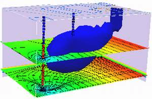
Sheetpile under a dam flownet#

Compare to the example shown on pp. 30-34.

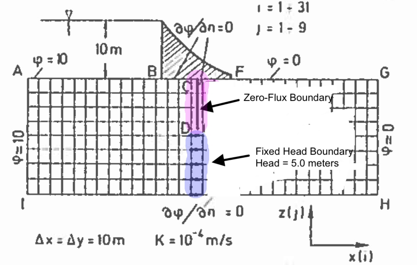
The figure below is a schematic of a dam built upon a permeable ground layer 80 meters thick (segment A to I).

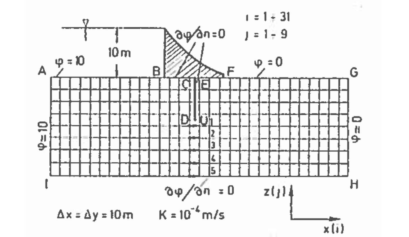
The dam has a base 60 meters long (segment B to F), with an upstream water depth of 10 meters. The downstream side of the dam is at 0 meters depth (otherwise its not a very good dam!). A sheetpile cutoff wall is installed beneath the dam (segment C to D to U to E). The ground layer has a hydraulic conductivity of K = 1 × 10−4 meters per second.

Important engineering questions are what is the pore water pressure under the dam, and is what is the total seepage under the dam? The pore water pressure can be found by solving for heads under the dam then subtracting the elevation of the computation location relative to a datum. The flow is found by Darcy’s law applied under the dam (shown as locations 1,2,3,4, and 5 in the sketch), which in turn requires computation of head under the dam. Thus the questions are answered by finding the head distribution under the dam.

The flow field (mathematically) extends an infinite distance upstream and downstream, but as a practical matter the contribution to seepage far upstream of the dam is negligible, and hence is approximated by the finite domain depicted.

Using the tools we have already we can simply build an input file, run our script and determine the head distribution (and thus compute the discharges under the dam. Then rerun with same script, but modify the boundary conditions and material properties to obtain the stream function - plot both solutions on the same contour map and viola we have a flownet.

The first is to represent the domain as shown, and make the following specifications in the boundary condition information, and we will treat the sheetpile cutoff wall as a low permeability inclusion (much like the the prior example). The boundary conditions are:

The segment from A to B is a constant head boundary with value equal to 10.
The segment from B to F is a zero-flux boundary.
The segment from B to C to D to U to E to F should be treated as a zero-flux boundary, but our mask does not extend into the interior – however the sheetpile itself can be approximated by providing a very small permeability. Alternately we could (should) modify the code to handle interior boundaries – but that is outside the scope of this chapter.
The segment from F to G is a constant head boundary with value equal to 0.
The segment form G to H is a constant head boundary with value equal to 0.
The segment from H to I is a zero-flux boundary.
The segment from I to A is a constant head boundary with value equal to 10.

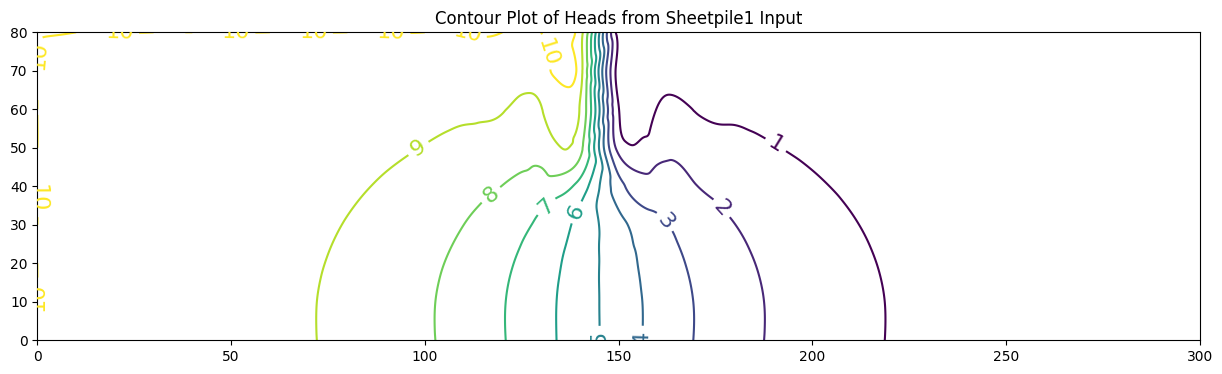
Here’s the input file for the heads $\phi$ in the picture

10
10
1
9
31
1e-12
5000
10 20 30 40 50 60 70 80 90 100 110 120 130 140 150 160 170 180 190 200 210 220 230 240 250 260 270 280 290 300
70 60 50 40 30 20 10 0
1 1 1 1 1 1 1 1 1 1 1 0 0 0 0 0 0 1 1 1 1 1 1 1 1 1 1 1 1 1
0 0 0 0 0 0 0 0 0 0 0 0 0 0 0 0 0 0 0 0 0 0 0 0 0 0 0 0 0 0
1 1 1 1 1 1 1 1
1 1 1 1 1 1 1 1
10 10 10 10 10 10 10 10 10 10 10 10 10 10 0 0 0 0 0 0 0 0 0 0 0 0 0 0 0 0
10 10 10 10 10 10 10 10 10 10 10 10 10 10 0 0 0 0 0 0 0 0 0 0 0 0 0 0 0 0
10 10 10 10 10 10 10 10 10 10 10 10 10 10 0 0 0 0 0 0 0 0 0 0 0 0 0 0 0 0
10 10 10 10 10 10 10 10 10 10 10 10 10 10 0 0 0 0 0 0 0 0 0 0 0 0 0 0 0 0
10 10 10 10 10 10 10 10 10 10 10 10 10 10 0 0 0 0 0 0 0 0 0 0 0 0 0 0 0 0
10 10 10 10 10 10 10 10 10 10 10 10 10 10 0 0 0 0 0 0 0 0 0 0 0 0 0 0 0 0
10 10 10 10 10 10 10 10 10 10 10 10 10 10 0 0 0 0 0 0 0 0 0 0 0 0 0 0 0 0
10 10 10 10 10 10 10 10 10 10 10 10 10 10 0 0 0 0 0 0 0 0 0 0 0 0 0 0 0 0
10 10 10 10 10 10 10 10 10 10 10 10 10 10 0 0 0 0 0 0 0 0 0 0 0 0 0 0 0 0
0001 0.0001 0.0001 0.0001 0.0001 0.0001 0.0001 0.0001 0.0001 0.0001 0.0001 0.0001 0.0001 0.0001 0.0000001 0.0000001 0.0001 0.0001 0.0001 0.0001 0.0001 0.0001 0.0001 0.0001 0.0001 0.0001 0.0001 0.0001 0.0001 0.0001 0.0001
0001 0.0001 0.0001 0.0001 0.0001 0.0001 0.0001 0.0001 0.0001 0.0001 0.0001 0.0001 0.0001 0.0001 0.0000001 0.0000001 0.0001 0.0001 0.0001 0.0001 0.0001 0.0001 0.0001 0.0001 0.0001 0.0001 0.0001 0.0001 0.0001 0.0001 0.0001
0001 0.0001 0.0001 0.0001 0.0001 0.0001 0.0001 0.0001 0.0001 0.0001 0.0001 0.0001 0.0001 0.0001 0.0000001 0.0000001 0.0001 0.0001 0.0001 0.0001 0.0001 0.0001 0.0001 0.0001 0.0001 0.0001 0.0001 0.0001 0.0001 0.0001 0.0001
0001 0.0001 0.0001 0.0001 0.0001 0.0001 0.0001 0.0001 0.0001 0.0001 0.0001 0.0001 0.0001 0.0001 0.0000001 0.0000001 0.0001 0.0001 0.0001 0.0001 0.0001 0.0001 0.0001 0.0001 0.0001 0.0001 0.0001 0.0001 0.0001 0.0001 0.0001
0001 0.0001 0.0001 0.0001 0.0001 0.0001 0.0001 0.0001 0.0001 0.0001 0.0001 0.0001 0.0001 0.0001 0.0000001 0.0000001 0.0001 0.0001 0.0001 0.0001 0.0001 0.0001 0.0001 0.0001 0.0001 0.0001 0.0001 0.0001 0.0001 0.0001 0.0001
0001 0.0001 0.0001 0.0001 0.0001 0.0001 0.0001 0.0001 0.0001 0.0001 0.0001 0.0001 0.0001 0.0001 0.0001 0.0001 0.0001 0.0001 0.0001 0.0001 0.0001 0.0001 0.0001 0.0001 0.0001 0.0001 0.0001 0.0001 0.0001 0.0001 0.0001
0001 0.0001 0.0001 0.0001 0.0001 0.0001 0.0001 0.0001 0.0001 0.0001 0.0001 0.0001 0.0001 0.0001 0.0001 0.0001 0.0001 0.0001 0.0001 0.0001 0.0001 0.0001 0.0001 0.0001 0.0001 0.0001 0.0001 0.0001 0.0001 0.0001 0.0001
0001 0.0001 0.0001 0.0001 0.0001 0.0001 0.0001 0.0001 0.0001 0.0001 0.0001 0.0001 0.0001 0.0001 0.0001 0.0001 0.0001 0.0001 0.0001 0.0001 0.0001 0.0001 0.0001 0.0001 0.0001 0.0001 0.0001 0.0001 0.0001 0.0001 0.0001
0001 0.0001 0.0001 0.0001 0.0001 0.0001 0.0001 0.0001 0.0001 0.0001 0.0001 0.0001 0.0001 0.0001 0.0001 0.0001 0.0001 0.0001 0.0001 0.0001 0.0001 0.0001 0.0001 0.0001 0.0001 0.0001 0.0001 0.0001 0.0001 0.0001 0.00010
0001 0.0001 0.0001 0.0001 0.0001 0.0001 0.0001 0.0001 0.0001 0.0001 0.0001 0.0001 0.0001 0.0001 0.0000001 0.0000001 0.0001 0.0001 0.0001 0.0001 0.0001 0.0001 0.0001 0.0001 0.0001 0.0001 0.0001 0.0001 0.0001 0.0001 0.0001
0001 0.0001 0.0001 0.0001 0.0001 0.0001 0.0001 0.0001 0.0001 0.0001 0.0001 0.0001 0.0001 0.0001 0.0000001 0.0000001 0.0001 0.0001 0.0001 0.0001 0.0001 0.0001 0.0001 0.0001 0.0001 0.0001 0.0001 0.0001 0.0001 0.0001 0.0001
0001 0.0001 0.0001 0.0001 0.0001 0.0001 0.0001 0.0001 0.0001 0.0001 0.0001 0.0001 0.0001 0.0001 0.0000001 0.0000001 0.0001 0.0001 0.0001 0.0001 0.0001 0.0001 0.0001 0.0001 0.0001 0.0001 0.0001 0.0001 0.0001 0.0001 0.0001
0001 0.0001 0.0001 0.0001 0.0001 0.0001 0.0001 0.0001 0.0001 0.0001 0.0001 0.0001 0.0001 0.0001 0.0000001 0.0000001 0.0001 0.0001 0.0001 0.0001 0.0001 0.0001 0.0001 0.0001 0.0001 0.0001 0.0001 0.0001 0.0001 0.0001 0.0001
0001 0.0001 0.0001 0.0001 0.0001 0.0001 0.0001 0.0001 0.0001 0.0001 0.0001 0.0001 0.0001 0.0001 0.0000001 0.0000001 0.0001 0.0001 0.0001 0.0001 0.0001 0.0001 0.0001 0.0001 0.0001 0.0001 0.0001 0.0001 0.0001 0.0001 0.0001
0001 0.0001 0.0001 0.0001 0.0001 0.0001 0.0001 0.0001 0.0001 0.0001 0.0001 0.0001 0.0001 0.0001 0.0001 0.0001 0.0001 0.0001 0.0001 0.0001 0.0001 0.0001 0.0001 0.0001 0.0001 0.0001 0.0001 0.0001 0.0001 0.0001 0.0001
0001 0.0001 0.0001 0.0001 0.0001 0.0001 0.0001 0.0001 0.0001 0.0001 0.0001 0.0001 0.0001 0.0001 0.0001 0.0001 0.0001 0.0001 0.0001 0.0001 0.0001 0.0001 0.0001 0.0001 0.0001 0.0001 0.0001 0.0001 0.0001 0.0001 0.0001
0001 0.0001 0.0001 0.0001 0.0001 0.0001 0.0001 0.0001 0.0001 0.0001 0.0001 0.0001 0.0001 0.0001 0.0001 0.0001 0.0001 0.0001 0.0001 0.0001 0.0001 0.0001 0.0001 0.0001 0.0001 0.0001 0.0001 0.0001 0.0001 0.0001 0.0001
0001 0.0001 0.0001 0.0001 0.0001 0.0001 0.0001 0.0001 0.0001 0.0001 0.0001 0.0001 0.0001 0.0001 0.0001 0.0001 0.0001 0.0001 0.0001 0.0001 0.0001 0.0001 0.0001 0.0001 0.0001 0.0001 0.0001 0.0001 0.0001 0.0001 0.0001

def sse(matrix1,matrix2):
    sse=0.0
    nr=len(matrix1) # get row count
    nc=len(matrix1[0]) # get column count
    for ir in range(nr):
        for jc in range(nc):
            sse=sse+(matrix1[ir][jc]-matrix2[ir][jc])**2
    return(sse)

def update(matrix1,matrix2):
    nr=len(matrix1) # get row count
    nc=len(matrix1[0]) # get column count
    ##print(nr,nc)
    for ir in range(nr):
        for jc in range(nc):
            ##print(ir,jc)
            matrix2[ir][jc]=matrix1[ir][jc]
    return(matrix2)

def writearray(matrix):
    nr=len(matrix) # get row count
    nc=len(matrix[0]) # get column count
    import numpy as np
    new_list = list(np.around(np.array(matrix), 3))    
    for ir in range(nr):
        print(ir,new_list[ir][:])
    return()

localfile = open("PotentialFnSheetpile1.txt","r") # connect and read file for 2D gw model
deltax = float(localfile.readline())
deltay = float(localfile.readline())
deltaz = float(localfile.readline())
nrows = int(localfile.readline())
ncols = int(localfile.readline())
tolerance = float(localfile.readline())
maxiter = int(localfile.readline())
distancex = [] # empty list
distancex.append([float(n) for n in localfile.readline().strip().split()])
distancey = [] # empty list
distancey.append([float(n) for n in localfile.readline().strip().split()])
boundarytop = [] #empty list
boundarytop.append([float(n) for n in localfile.readline().strip().split()])
boundarybottom = [] #empty list
boundarybottom.append([int(n) for n in localfile.readline().strip().split()])
boundaryleft = [] #empty list
boundaryleft.append([int(n) for n in localfile.readline().strip().split()])
boundaryright = [] #empty list
boundaryright.append([int(n) for n in localfile.readline().strip().split()])
head =[] # empty list
for irow in range(nrows):
        head.append([float(n) for n in localfile.readline().strip().split()])
hydcondx = [] # empty list
for irow in range(nrows):
        hydcondx.append([float(n) for n in localfile.readline().strip().split()])
hydcondy = [] # empty list
for irow in range(nrows):
        hydcondy.append([float(n) for n in localfile.readline().strip().split()])
localfile.close() # Disconnect the file
##
amat = [[0 for j in range(ncols)] for i in range(nrows)]
bmat = [[0 for j in range(ncols)] for i in range(nrows)]
cmat = [[0 for j in range(ncols)] for i in range(nrows)]
dmat = [[0 for j in range(ncols)] for i in range(nrows)]
##
for irow in range(1,nrows-1):
    for jcol in range(1,ncols-1):
        amat[irow][jcol] = (( hydcondx[irow-1][jcol  ]+ hydcondx[irow  ][jcol  ]) * deltaz ) /(2.0*deltax**2)
        bmat[irow][jcol] = (( hydcondx[irow  ][jcol  ]+ hydcondx[irow+1][jcol  ]) * deltaz ) /(2.0*deltax**2)
        cmat[irow][jcol] = (( hydcondy[irow  ][jcol-1]+ hydcondy[irow  ][jcol  ]) * deltaz ) /(2.0*deltay**2)
        dmat[irow][jcol] = (( hydcondy[irow  ][jcol  ]+ hydcondy[irow  ][jcol+1]) * deltaz ) /(2.0*deltay**2)
##
headold = [[0 for jc in range(ncols)] for ir in range(nrows)] #force new matrix
headold = update(head,headold) # update
##writearray(head)
##print("----")
##writearray(headold)
##print("--------")
tolflag = False
for iter in range(maxiter):
##    print("begin iteration")
##    writearray(head)
##    print("----")
##    writearray(headold)
##    print("--------")

# Boundary Conditions

# first and last row special == no flow boundaries
    for jcol in range(ncols):
        if boundarytop[0][jcol] == 0: # no - flow at top
            head [0][jcol ] = head[1][jcol ]
        if boundarybottom[0][ jcol ] == 0: # no - flow at bottom
            head [nrows-1][jcol ] = head[nrows-2][jcol ]
# first and last column special == no flow boundaries     
    for irow in range(nrows): 
        if  boundaryleft[0][ irow ] == 0:
            head[irow][0] = head [irow][1] # no - flow at left
        if boundaryright[0][ irow ] == 0: 
            head [irow][ncols-1] = head[ irow ][ncols-2] # no - flow at right
# interior updates
    for irow in range(1,nrows-1):
        for jcol in range(1,ncols-1):
            head[irow][jcol]=( amat[irow][jcol]*head[irow-1][jcol  ] 
                              +bmat[irow][jcol]*head[irow+1][jcol  ] 
                              +cmat[irow][jcol]*head[irow  ][jcol-1] 
                              +dmat[irow][jcol]*head[irow  ][jcol+1])/(amat[ irow][jcol ]+ bmat[ irow][jcol ]+ cmat[ irow][jcol ]+ dmat[ irow][jcol ])
# test for stopping iterations
##    print("end iteration")
##    writearray(head)
##    print("----")
##    writearray(headold)
    percentdiff = sse(head,headold)
    if  percentdiff <= tolerance:
        print("Exit iterations in velocity potential because tolerance met ")
        print("Iterations =" , iter+1 ) ;
        tolflag = True
        break
    headold = update(head,headold)
print("End Calculations")
print("Iterations    = ",iter+1)
print("Closure Error = ",round(percentdiff,3))
print("Head Map")
print("----")
writearray(head)
print("----")
############# Contour Plot
my_xyz = [] # empty list
for irow in range(nrows):
    for jcol in range(ncols):
        my_xyz.append([distancex[0][jcol],distancey[0][irow],head[irow][jcol]])
import pandas
my_xyz = pandas.DataFrame(my_xyz) # convert into a data frame
#print(my_xyz) # activate to examine the dataframe
import numpy 
import matplotlib.pyplot
from scipy.interpolate import griddata
# extract lists from the dataframe
coord_x = my_xyz[0].values.tolist() # column 0 of dataframe
coord_y = my_xyz[1].values.tolist() # column 1 of dataframe
coord_z = my_xyz[2].values.tolist() # column 2 of dataframe
coord_xy = numpy.column_stack((coord_x, coord_y))
# Set plotting range in original data units
lon = numpy.linspace(min(coord_x), max(coord_x), 3000)
lat = numpy.linspace(min(coord_y), max(coord_y), 800)
X, Y = numpy.meshgrid(lon, lat)
# Grid the data; use linear interpolation (choices are nearest, linear, cubic)
Z = griddata(numpy.array(coord_xy), numpy.array(coord_z), (X, Y), method='cubic')
# Build the map
fig, ax = matplotlib.pyplot.subplots()
fig.set_size_inches(15, 4)
levels1 = [1,2,3,4,5,6,7,8,9,10]
CS = ax.contour(X, Y, Z, levels1)
ax.clabel(CS, inline=2, fontsize=16)
ax.set_title('Contour Plot of Heads from Sheetpile1 Input')

Exit iterations in velocity potential because tolerance met 
Iterations = 443
End Calculations
Iterations    =  443
Closure Error =  0.0
Head Map
----

[10.    10.    10.    10.    10.    10.    10.    10.    10.    10.
   10.    10.    10.     9.478  0.524  0.     0.     0.     0.
    0.     0.     0.     0.     0.     0.     0.     0.     0.
  ]
[10.     9.98   9.959  9.936  9.91   9.881  9.848  9.808  9.763  9.71
652  9.591  9.535  9.497  9.478  0.524  0.505  0.467  0.411  0.351
293  0.241  0.196  0.157  0.125  0.097  0.073  0.052  0.034  0.016
  ]
[10.     9.96   9.919  9.874  9.824  9.767  9.701  9.623  9.532  9.426
306  9.178  9.054  8.965  8.949  1.055  1.039  0.95   0.827  0.699
58   0.475  0.385  0.309  0.244  0.19   0.143  0.102  0.066  0.032
  ]
[10.     9.943  9.883  9.818  9.746  9.663  9.566  9.451  9.316  9.156
969  8.759  8.538  8.351  8.336  1.67   1.654  1.468  1.247  1.038
852  0.694  0.56   0.448  0.354  0.275  0.207  0.148  0.095  0.047
  ]
[10.     9.927  9.852  9.77   9.678  9.572  9.448  9.3    9.124  8.912
657  8.351  7.986  7.559  6.629  3.379  2.448  2.021  1.657  1.352
098  0.888  0.714  0.57   0.45   0.348  0.262  0.187  0.121  0.059
  ]
[10.     9.915  9.827  9.731  9.623  9.499  9.353  9.179  8.968  8.711
395  8.002  7.498  6.806  5.702  4.307  3.202  2.511  2.007  1.615
301  1.046  0.838  0.667  0.526  0.407  0.306  0.219  0.141  0.069
  ]
[10.     9.907  9.81   9.704  9.586  9.448  9.287  9.093  8.858  8.569
212  7.764  7.196  6.465  5.528  4.48   3.544  2.813  2.246  1.8
444  1.158  0.926  0.736  0.579  0.448  0.337  0.24   0.155  0.076
  ]
[10.     9.903  9.801  9.69   9.566  9.422  9.253  9.049  8.801  8.496
118  7.647  7.057  6.33   5.467  4.542  3.679  2.952  2.364  1.894
518  1.215  0.971  0.771  0.606  0.469  0.352  0.251  0.162  0.079
  ]
[10.     9.903  9.801  9.69   9.566  9.422  9.253  9.049  8.801  8.496
118  7.647  7.057  6.33   5.467  4.542  3.679  2.952  2.364  1.894
518  1.215  0.971  0.771  0.606  0.469  0.352  0.251  0.162  0.079
  ]
----

Text(0.5, 1.0, 'Contour Plot of Heads from Sheetpile1 Input')

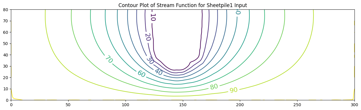
../../_images/b63403a92c82f504bf963242af37c59ee153f12018bf1f24073ba672a6c0e530.png

Now we reuse the code, but change head to stream and modify the contour plot variable names as well as modify the input file to reflect the changed material properties and boundary conditions.

Here’s the input file for the stream function

10
10
1
9
31
1e-12
5000
10 20 30 40 50 60 70 80 90 100 110 120 130 140 150 160 170 180 190 200 210 220 230 240 250 260 270 280 290 300
70 60 50 40 30 20 10 0
0 0 0 0 0 0 0 0 0 0 0 0 0 1 1 0 0 0 0 0 0 0 0 0 0 0 0 0 0 0
1 1 1 1 1 1 1 1 1 1 1 1 1 1 1 1 1 1 1 1 1 1 1 1 1 1 1 1 1 1
1 1 1 1 1 1 1 1
1 1 1 1 1 1 1 1
0 0 0 0 0 0 0 0 0 0 0 0 0 0 0 0 0 0 0 0 0 0 0 0 0 0 0 0 0 100
0 0 0 0 0 0 0 0 0 0 0 0 0 0 0 0 0 0 0 0 0 0 0 0 0 0 0 0 0 100
0 0 0 0 0 0 0 0 0 0 0 0 0 0 0 0 0 0 0 0 0 0 0 0 0 0 0 0 0 100
0 0 0 0 0 0 0 0 0 0 0 0 0 0 0 0 0 0 0 0 0 0 0 0 0 0 0 0 0 100
0 0 0 0 0 0 0 0 0 0 0 0 0 0 0 0 0 0 0 0 0 0 0 0 0 0 0 0 0 100
0 0 0 0 0 0 0 0 0 0 0 0 0 0 0 0 0 0 0 0 0 0 0 0 0 0 0 0 0 100
0 0 0 0 0 0 0 0 0 0 0 0 0 0 0 0 0 0 0 0 0 0 0 0 0 0 0 0 0 100
0 0 0 0 0 0 0 0 0 0 0 0 0 0 0 0 0 0 0 0 0 0 0 0 0 0 0 0 0 100
100 100 100 100 100 100 100 100 100 100 100 100 100 100 100 100 100 100 100 100 100 100 100 100 100 100 100 100 100 100
10000 10000 10000 10000 10000 10000 10000 10000 10000 10000 10000 10000 10000 10000000 10000000 10000 10000 10000 10000 10000 10000 10000 10000 10000 10000 10000 10000 10000 10000 10000
10000 10000 10000 10000 10000 10000 10000 10000 10000 10000 10000 10000 10000 10000000 10000000 10000 10000 10000 10000 10000 10000 10000 10000 10000 10000 10000 10000 10000 10000 10000
10000 10000 10000 10000 10000 10000 10000 10000 10000 10000 10000 10000 10000 10000000 10000000 10000 10000 10000 10000 10000 10000 10000 10000 10000 10000 10000 10000 10000 10000 10000
10000 10000 10000 10000 10000 10000 10000 10000 10000 10000 10000 10000 10000 10000000 10000000 10000 10000 10000 10000 10000 10000 10000 10000 10000 10000 10000 10000 10000 10000 10000
10000 10000 10000 10000 10000 10000 10000 10000 10000 10000 10000 10000 10000 10000000 10000000 10000 10000 10000 10000 10000 10000 10000 10000 10000 10000 10000 10000 10000 10000 10000
10000 10000 10000 10000 10000 10000 10000 10000 10000 10000 10000 10000 10000 10000 10000 10000 10000 10000 10000 10000 10000 10000 10000 10000 10000 10000 10000 10000 10000 10000
10000 10000 10000 10000 10000 10000 10000 10000 10000 10000 10000 10000 10000 10000 10000 10000 10000 10000 10000 10000 10000 10000 10000 10000 10000 10000 10000 10000 10000 10000
10000 10000 10000 10000 10000 10000 10000 10000 10000 10000 10000 10000 10000 10000 10000 10000 10000 10000 10000 10000 10000 10000 10000 10000 10000 10000 10000 10000 10000 10000
10000 10000 10000 10000 10000 10000 10000 10000 10000 10000 10000 10000 10000 10000 10000 10000 10000 10000 10000 10000 10000 10000 10000 10000 10000 10000 10000 10000 10000 100000
10000 10000 10000 10000 10000 10000 10000 10000 10000 10000 10000 10000 10000 10000000 10000000 10000 10000 10000 10000 10000 10000 10000 10000 10000 10000 10000 10000 10000 10000 10000
10000 10000 10000 10000 10000 10000 10000 10000 10000 10000 10000 10000 10000 10000000 10000000 10000 10000 10000 10000 10000 10000 10000 10000 10000 10000 10000 10000 10000 10000 10000
10000 10000 10000 10000 10000 10000 10000 10000 10000 10000 10000 10000 10000 10000000 10000000 10000 10000 10000 10000 10000 10000 10000 10000 10000 10000 10000 10000 10000 10000 10000
10000 10000 10000 10000 10000 10000 10000 10000 10000 10000 10000 10000 10000 10000000 10000000 10000 10000 10000 10000 10000 10000 10000 10000 10000 10000 10000 10000 10000 10000 10000
10000 10000 10000 10000 10000 10000 10000 10000 10000 10000 10000 10000 10000 10000000 10000000 10000 10000 10000 10000 10000 10000 10000 10000 10000 10000 10000 10000 10000 10000 10000
10000 10000 10000 10000 10000 10000 10000 10000 10000 10000 10000 10000 10000 10000 10000 10000 10000 10000 10000 10000 10000 10000 10000 10000 10000 10000 10000 10000 10000 10000
10000 10000 10000 10000 10000 10000 10000 10000 10000 10000 10000 10000 10000 10000 10000 10000 10000 10000 10000 10000 10000 10000 10000 10000 10000 10000 10000 10000 10000 10000
10000 10000 10000 10000 10000 10000 10000 10000 10000 10000 10000 10000 10000 10000 10000 10000 10000 10000 10000 10000 10000 10000 10000 10000 10000 10000 10000 10000 10000 10000
10000 10000 10000 10000 10000 10000 10000 10000 10000 10000 10000 10000 10000 10000 10000 10000 10000 10000 10000 10000 10000 10000 10000 10000 10000 10000 10000 10000 10000 10000

In these examples the value of the stream function is arbitrarily set to range from $0$ to $100$. One useful interpretation of stream function values is that their differences indicate the flow fraction (of total flow) that flows between the streamlines (contour lines of constant stream function value).

def sse(matrix1,matrix2):
    sse=0.0
    nr=len(matrix1) # get row count
    nc=len(matrix1[0]) # get column count
    for ir in range(nr):
        for jc in range(nc):
            sse=sse+(matrix1[ir][jc]-matrix2[ir][jc])**2
    return(sse)

def update(matrix1,matrix2):
    nr=len(matrix1) # get row count
    nc=len(matrix1[0]) # get column count
    ##print(nr,nc)
    for ir in range(nr):
        for jc in range(nc):
            ##print(ir,jc)
            matrix2[ir][jc]=matrix1[ir][jc]
    return(matrix2)

def writearray(matrix):
    nr=len(matrix) # get row count
    nc=len(matrix[0]) # get column count
    import numpy as np
    new_list = list(np.around(np.array(matrix), 3))    
    for ir in range(nr):
        print(ir,new_list[ir][:])
    return()

localfile = open("StreamFnSheetpile1.txt","r") # connect and read file for 2D gw model
deltax = float(localfile.readline())
deltay = float(localfile.readline())
deltaz = float(localfile.readline())
nrows = int(localfile.readline())
ncols = int(localfile.readline())
tolerance = float(localfile.readline())
maxiter = int(localfile.readline())
distancex = [] # empty list
distancex.append([float(n) for n in localfile.readline().strip().split()])
distancey = [] # empty list
distancey.append([float(n) for n in localfile.readline().strip().split()])
boundarytop = [] #empty list
boundarytop.append([float(n) for n in localfile.readline().strip().split()])
boundarybottom = [] #empty list
boundarybottom.append([int(n) for n in localfile.readline().strip().split()])
boundaryleft = [] #empty list
boundaryleft.append([int(n) for n in localfile.readline().strip().split()])
boundaryright = [] #empty list
boundaryright.append([int(n) for n in localfile.readline().strip().split()])
stream =[] # empty list
for irow in range(nrows):
        stream.append([float(n) for n in localfile.readline().strip().split()])
hydcondx = [] # empty list
for irow in range(nrows):
        hydcondx.append([float(n) for n in localfile.readline().strip().split()])
hydcondy = [] # empty list
for irow in range(nrows):
        hydcondy.append([float(n) for n in localfile.readline().strip().split()])
localfile.close() # Disconnect the file
##
amat = [[0 for j in range(ncols)] for i in range(nrows)]
bmat = [[0 for j in range(ncols)] for i in range(nrows)]
cmat = [[0 for j in range(ncols)] for i in range(nrows)]
dmat = [[0 for j in range(ncols)] for i in range(nrows)]
##
for irow in range(1,nrows-1):
    for jcol in range(1,ncols-1):
        amat[irow][jcol] = (( hydcondx[irow-1][jcol  ]+ hydcondx[irow  ][jcol  ]) * deltaz ) /(2.0*deltax**2)
        bmat[irow][jcol] = (( hydcondx[irow  ][jcol  ]+ hydcondx[irow+1][jcol  ]) * deltaz ) /(2.0*deltax**2)
        cmat[irow][jcol] = (( hydcondy[irow  ][jcol-1]+ hydcondy[irow  ][jcol  ]) * deltaz ) /(2.0*deltay**2)
        dmat[irow][jcol] = (( hydcondy[irow  ][jcol  ]+ hydcondy[irow  ][jcol+1]) * deltaz ) /(2.0*deltay**2)
##
streamold = [[0 for jc in range(ncols)] for ir in range(nrows)] #force new matrix
streamold = update(stream,streamold) # update
##writearray(stream)
##print("----")
##writearray(streamold)
##print("--------")
tolflag = False
for iter in range(maxiter):
##    print("begin iteration")
##    writearray(stream)
##    print("----")
##    writearray(streamold)
##    print("--------")

# Boundary Conditions

# first and last row special == no flow boundaries
    for jcol in range(ncols):
        if boundarytop[0][jcol] == 0: # no - flow at top
            stream [0][jcol ] = stream[1][jcol ]
        if boundarybottom[0][ jcol ] == 0: # no - flow at bottom
            stream [nrows-1][jcol ] = stream[nrows-2][jcol ]
# first and last column special == no flow boundaries     
    for irow in range(nrows): 
        if  boundaryleft[0][ irow ] == 0:
            stream[irow][0] = stream [irow][1] # no - flow at left
        if boundaryright[0][ irow ] == 0: 
            stream [irow][ncols-1] = stream[ irow ][ncols-2] # no - flow at right
# interior updates
    for irow in range(1,nrows-1):
        for jcol in range(1,ncols-1):
            stream[irow][jcol]=( amat[irow][jcol]*stream[irow-1][jcol  ] 
                              +bmat[irow][jcol]*stream[irow+1][jcol  ] 
                              +cmat[irow][jcol]*stream[irow  ][jcol-1] 
                              +dmat[irow][jcol]*stream[irow  ][jcol+1])/(amat[ irow][jcol ]+ bmat[ irow][jcol ]+ cmat[ irow][jcol ]+ dmat[ irow][jcol ])
# test for stopping iterations
##    print("end iteration")
##    writearray(stream)
##    print("----")
##    writearray(streamold)
    percentdiff = sse(stream,streamold)
    if  percentdiff <= tolerance:
        print("Exit iterations in Stream Function because tolerance met ")
        print("Iterations =" , iter+1 ) ;
        tolflag = True
        break
    streamold = update(stream,streamold)
print("End Calculations")
print("Iterations    = ",iter+1)
print("Closure Error = ",round(percentdiff,3))
print("Stream Function Map")
print("----")
writearray(stream)
print("----")
####################### Contour Plot ###############
my_xyz2 = [] # empty list
for irow in range(nrows):
    for jcol in range(ncols):
        my_xyz2.append([distancex[0][jcol],distancey[0][irow],stream[irow][jcol]])
import pandas
my_xyz2 = pandas.DataFrame(my_xyz2) # convert into a data frame
#print(my_xyz) # activate to examine the dataframe
import numpy 
import matplotlib.pyplot
from scipy.interpolate import griddata
# extract lists from the dataframe
coord_x2 = my_xyz2[0].values.tolist() # column 0 of dataframe
coord_y2 = my_xyz2[1].values.tolist() # column 1 of dataframe
coord_z2 = my_xyz2[2].values.tolist() # column 2 of dataframe
coord_xy2 = numpy.column_stack((coord_x2, coord_y2))
# Set plotting range in original data units
lon = numpy.linspace(min(coord_x2), max(coord_x2), 3000)
lat = numpy.linspace(min(coord_y2), max(coord_y2), 800)
X2, Y2 = numpy.meshgrid(lon, lat)
# Grid the data; use linear interpolation (choices are nearest, linear, cubic)
Z2 = griddata(numpy.array(coord_xy2), numpy.array(coord_z2), (X2, Y2), method='cubic')
# Build the map
fig, ax = matplotlib.pyplot.subplots()
fig.set_size_inches(15, 4)
levels = [10,20,30,40,50,60,70,80,90,100]
CS2 = ax.contour(X2, Y2, Z2, levels )
ax.clabel(CS2, inline=2, fontsize=16)
ax.set_title('Contour Plot of Stream Function for Sheetpile1 Input')

Exit iterations in Stream Function because tolerance met 
Iterations = 396
End Calculations
Iterations    =  396
Closure Error =  0.0
Stream Function Map
----
[100.     96.845  93.555  89.987  85.989  81.394  76.015  69.642  62.046
99   42.26   29.74   15.542   0.191   0.      0.      0.19   15.469
592  42.031  52.669  61.62   69.093  75.318  80.519  84.898  88.632
878  94.773  97.442 100.   ]
[100.     96.845  93.555  89.987  85.989  81.394  76.015  69.642  62.046
99   42.26   29.74   15.542   0.191   0.16    0.16    0.19   15.469
592  42.031  52.669  61.62   69.093  75.318  80.519  84.898  88.632
878  94.773  97.442 100.   ]
[100.     96.982  93.832  90.416  86.586  82.178  77.008  70.865  63.507
663  44.05   31.419  16.694   0.337   0.304   0.304   0.336  16.625
277  43.83   54.356  63.099  70.34   76.342  81.342  85.543  89.121
229  94.999  97.553 100.   ]
[100.     97.249  94.377  91.26   87.76   83.724  78.976  73.304  66.452
105  47.859  35.19   19.48    0.47    0.432   0.432   0.47   19.416
061  47.658  57.826  66.081  72.825  78.369  82.963  86.81   90.08
916  95.443  97.77  100.   ]
[100.     97.636  95.168  92.486  89.47   85.984  81.867  76.921  70.894
447  54.089  42.004  25.566   0.634   0.541   0.541   0.634  25.509
891  53.916  63.207  70.575  76.51   81.346  85.33   88.655  91.473
914  96.085  98.085 100.   ]
[100.     98.128  96.172  94.045  91.65   88.875  85.587  81.619  76.754
701  63.045  53.171  40.146  22.721   0.665   0.665  22.703  40.095
079  62.907  70.511  76.502  81.294  85.175  88.358  91.005  93.244
18   96.901  98.484 100.   ]
[100.     98.703  97.348  95.872  94.209  92.279  89.987  87.213  83.804
559  74.22   67.487  59.128  49.437  40.688  40.683  49.419  59.09
422  74.124  79.426  83.629  86.988  89.702  91.921  93.763  95.318
661  97.853  98.95  100.   ]
[100.     99.336  98.643  97.888  97.036  96.046  94.869  93.443  91.689
509  86.79   83.43   79.442  75.211  71.965  71.962  75.201  79.422
396  86.74   89.442  91.6    93.328  94.723  95.863  96.808  97.604
292  98.902  99.463 100.   ]
[100. 100. 100. 100. 100. 100. 100. 100. 100. 100. 100. 100. 100. 100.
100. 100. 100. 100. 100. 100. 100. 100. 100. 100. 100. 100. 100.
100. 100.]
----

Text(0.5, 1.0, 'Contour Plot of Stream Function for Sheetpile1 Input')

../../_images/415fadf0c7d84324bb476438fbd9a4f4c6c652f50de3515eba5d08db838e5236.png

Now both plots on same canvass

# Head (Velocity Potential Map)
# Grid the data; use linear interpolation (choices are nearest, linear, cubic)
Z = griddata(numpy.array(coord_xy), numpy.array(coord_z), (X, Y), method='cubic')
Z2 = griddata(numpy.array(coord_xy2), numpy.array(coord_z2), (X2, Y2), method='cubic')
# Build the map
fig, ax = matplotlib.pyplot.subplots()
fig.set_size_inches(15, 4)
levels1 = [1,2,3,4,5,6,7,8,9]
CS = ax.contour(X, Y, Z, levels1)
levels2 = [10,20,30,40,50,60,70,80,90]
CS2 = ax.contour(X2, Y2, Z2, levels2 )
ax.clabel(CS, inline=2, fontsize=12)
ax.clabel(CS2, inline=2, fontsize=12)
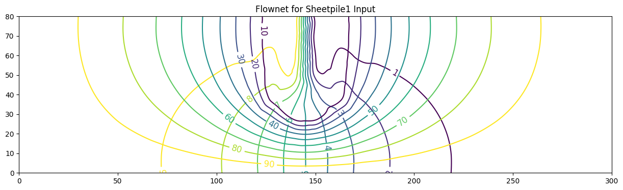
ax.set_title('Flownet for Sheetpile1 Input')

Text(0.5, 1.0, 'Flownet for Sheetpile1 Input')

../../_images/b1ef8ba8490c511df09c6db9c86ffa09e7fbfbb2af21f2763d6bfa59d8f8e3e7.png

Tip

Using AI to improve your (already working) code: a practical framework Goal: keep your code correct, make it clearer/faster/safer—and learn something in the process.

Set the ground rules (before you paste code)

Snapshot a baseline: save the working script + sample inputs/outputs.

State objectives: e.g., “modularize,” “add tests,” “speed up by 2×,” “remove globals.”

List invariants: what must not change (I/O format, algorithm, results within tolerance).

Share minimal context: problem description, performance pain points, constraints (no new deps, Py≥3.10, runs headless, etc.).

Provide a small, runnable example: tiny input + expected output for quick checks.

Ask for a plan, then patches

First request: “Propose a refactor plan with milestones (interfaces, tests, perf check).”

Work in small steps (e.g., extract functions → add dataclasses → add tests → add CLI).

Prefer diffs or focused snippets over full rewrites to avoid regressions.

Build safety nets

Tests: ask for unit tests (edge cases + typical), fixtures, and a quick benchmark harness.

Determinism: specify seeds and tolerances (e.g., atol=1e-6), and record environment info.

Validation hooks: print/plot key diagnostics to confirm physics/logic after each change.

Check the work

Require a short rationale for each change (why it helps; complexity trade-offs).

Watch for red flags: invented APIs, silent dependency creep, algorithm swaps, huge boilerplate.

Inspect performance: time/memory before vs after; accept only measurable wins.

Document and package

Ask for docstrings, type hints, and a concise README (usage, assumptions, limits).

Ensure error messages guide the user; add logging where it helps debugging.

Keep your license/copyright headers intact.

Prompt templates (copy/paste)

“Refactor into a module with read_input, assemble_coeffs, solve, plot. Keep I/O identical.”

“Add dataclasses for grid/boundaries; no new dependencies; include type hints.”

“Write pytest tests for 3 cases (baseline, edge, heterogeneity); set numeric tolerances.”

“Suggest a safe SOR acceleration (ω selection), show where it slots in, and guard with a flag.”

“Produce a minimal benchmark script and report speedup on the provided sample.”

Remember: AI is a pair programmer, not an oracle. Keep runs tight, verify often, and merge improvements only when they pass your tests and preserve the science.

What follows below are two modules saved as .py files which are loaded in an identical fashion as a library or any other python module. As you shall observe they make the model build/display much more tidy. They implement the algorithm identically, but are modular.

I supplied the code above with the following prompt:

Attached is my potential flow code. Can you refactor into logical modules, and enforce best programming practices. As this is pedagogical - error checking is not vital, but elegant fails are desirable.

The results are two modules potential_flow_mod.py and flownet_plotter.py

potential_flow_mod.py

# potential_flow_mod.py
#
# Built collaboratively by Sensei and OpenAI ChatGPT on 2025-08-14;
# Derived from the classroom “PotentialFnSheetpile1” script.
# Gauss–Seidel iterative solver for Laplacian-type linear systems (in-place updates)
#
from dataclasses import dataclass
from typing import Tuple
import numpy as np
import matplotlib.pyplot as plt
from scipy.interpolate import griddata

@dataclass
class GridSpec:
    deltax: float
    deltay: float
    deltaz: float
    nrows: int
    ncols: int
    distancex: np.ndarray
    distancey: np.ndarray

@dataclass
class Boundaries:
    top: np.ndarray
    bottom: np.ndarray
    left: np.ndarray
    right: np.ndarray

@dataclass
class ModelData:
    grid: GridSpec
    bounds: Boundaries
    head0: np.ndarray
    Kx: np.ndarray
    Ky: np.ndarray
    tolerance: float
    maxiter: int

def read_potential_input(path: str) -> ModelData:
    with open(path, "r") as f:
        deltax = float(f.readline().strip())
        deltay = float(f.readline().strip())
        deltaz = float(f.readline().strip())
        nrows = int(f.readline().strip())
        ncols = int(f.readline().strip())
        tolerance = float(f.readline().strip())
        maxiter = int(f.readline().strip())

        distancex = np.array([float(x) for x in f.readline().strip().split()], dtype=float)
        distancey = np.array([float(y) for y in f.readline().strip().split()], dtype=float)

        boundarytop = np.array([float(v) for v in f.readline().strip().split()], dtype=float)
        boundarybottom = np.array([int(v) for v in f.readline().strip().split()], dtype=int)
        boundaryleft = np.array([int(v) for v in f.readline().strip().split()], dtype=int)
        boundaryright = np.array([int(v) for v in f.readline().strip().split()], dtype=int)

        head0 = np.zeros((nrows, ncols), dtype=float)
        for i in range(nrows):
            head0[i, :] = np.array([float(v) for v in f.readline().strip().split()], dtype=float)

        Kx = np.zeros((nrows, ncols), dtype=float)
        for i in range(nrows):
            Kx[i, :] = np.array([float(v) for v in f.readline().strip().split()], dtype=float)

        Ky = np.zeros((nrows, ncols), dtype=float)
        for i in range(nrows):
            Ky[i, :] = np.array([float(v) for v in f.readline().strip().split()], dtype=float)

    grid = GridSpec(deltax, deltay, deltaz, nrows, ncols, distancex, distancey)
    bounds = Boundaries(boundarytop, boundarybottom, boundaryleft, boundaryright)
    return ModelData(grid, bounds, head0, Kx, Ky, tolerance, maxiter)

def assemble_coefficients(Kx: np.ndarray, Ky: np.ndarray, grid: GridSpec):
    nr, nc = grid.nrows, grid.ncols
    A = np.zeros((nr, nc), dtype=float)
    B = np.zeros((nr, nc), dtype=float)
    C = np.zeros((nr, nc), dtype=float)
    D = np.zeros((nr, nc), dtype=float)
    dx2 = grid.deltax ** 2
    dy2 = grid.deltay ** 2
    dz = grid.deltaz
    for i in range(1, nr - 1):
        for j in range(1, nc - 1):
            A[i, j] = ((Kx[i - 1, j] + Kx[i, j]) * dz) / (2.0 * dx2)
            B[i, j] = ((Kx[i, j] + Kx[i + 1, j]) * dz) / (2.0 * dx2)
            C[i, j] = ((Ky[i, j - 1] + Ky[i, j]) * dz) / (2.0 * dy2)
            D[i, j] = ((Ky[i, j] + Ky[i, j + 1]) * dz) / (2.0 * dy2)
    return A, B, C, D

def apply_no_flow_edges(head: np.ndarray, bounds: Boundaries) -> None:
    nr, nc = head.shape
    for j in range(nc):
        if bounds.top[j] == 0:
            head[0, j] = head[1, j]
        if bounds.bottom[j] == 0:
            head[nr - 1, j] = head[nr - 2, j]
    for i in range(nr):
        if bounds.left[i] == 0:
            head[i, 0] = head[i, 1]
        if bounds.right[i] == 0:
            head[i, nc - 1] = head[i, nc - 2]

def gauss_seidel_sweep(head: np.ndarray, A: np.ndarray, B: np.ndarray, C: np.ndarray, D: np.ndarray) -> None:
    nr, nc = head.shape
    for i in range(1, nr - 1):
        for j in range(1, nc - 1):
            wsum = A[i, j] + B[i, j] + C[i, j] + D[i, j]
            if wsum > 0.0:
                head[i, j] = (
                    A[i, j] * head[i - 1, j] +
                    B[i, j] * head[i + 1, j] +
                    C[i, j] * head[i, j - 1] +
                    D[i, j] * head[i, j + 1]
                ) / wsum

def solve_potential(model, verbose: bool = True):
    grid, bounds = model.grid, model.bounds
    head = model.head0.copy()
    head_old = head.copy()
    A, B, C, D = assemble_coefficients(model.Kx, model.Ky, grid)
    tol = model.tolerance
    maxiter = model.maxiter
    for it in range(1, maxiter + 1):
        apply_no_flow_edges(head, bounds)
        gauss_seidel_sweep(head, A, B, C, D)
        sse = float(np.sum((head - head_old) ** 2))
        if verbose and (it % 50 == 0 or it == 1):
            print(f"Iter {it:6d} | SSE={sse:.6e}")
        if sse <= tol:
            if verbose:
                print("Exit iterations in velocity potential because tolerance met")
                print("Iterations =", it)
            return head, it, sse
        head_old[:, :] = head
    if verbose:
        print("Reached max iterations.")
    return head, maxiter, float(np.sum((head - head_old) ** 2))

def plot_head_contours(distancex: np.ndarray, distancey: np.ndarray, head: np.ndarray,
                       title: str = "Contour Plot of Heads", nx: int = 1200, ny: int = 600, method: str = "cubic"):
    Xpts, Ypts = np.meshgrid(distancex, distancey)
    pts = np.column_stack([Xpts.ravel(), Ypts.ravel()])
    vals = head.ravel()
    gx = np.linspace(distancex.min(), distancex.max(), nx)
    gy = np.linspace(distancey.min(), distancey.max(), ny)
    GX, GY = np.meshgrid(gx, gy)
    GZ = griddata(pts, vals, (GX, GY), method=method)
    fig, ax = plt.subplots(figsize=(12, 4))
    CS = ax.contour(GX, GY, GZ, levels=10)
    ax.clabel(CS, inline=2, fontsize=12)
    ax.set_title(title)
    ax.set_xlabel("x (distance units)")
    ax.set_ylabel("y (distance units)")
    fig.tight_layout()
    return fig

flownet_plotter.py

# flownet_plotter.py
#
# Built collaboratively by Sensei and OpenAI ChatGPT on 2025-08-14.
# Overlays equipotential (head) and stream-function contours on a common grid to form a flownet.
# Reads two 3-column XYZ files (x y value), grids via scipy.griddata, and plots head (solid) + stream (dashed).
# Includes a helper to write XYZ from regular grids and a CLI for quick use; no explicit colors are set.
#
import numpy as np
import matplotlib.pyplot as plt
from scipy.interpolate import griddata
from matplotlib.lines import Line2D
import argparse
import os

def read_xyz(path):
    """
    Read an XYZ file with 3 columns: x, y, value.
    Delimiters may be commas or whitespace.
    Lines starting with '#' or '//' are ignored.
    Returns: (x, y, z) as 1D numpy arrays.
    """
    xs, ys, zs = [], [], []
    with open(path, 'r', encoding='utf-8') as f:
        for line in f:
            s = line.strip()
            if not s:
                continue
            if s.startswith('#') or s.startswith('//'):
                continue
            s = s.replace(',', ' ')
            parts = s.split()
            if len(parts) < 3:
                continue
            try:
                x, y, z = float(parts[0]), float(parts[1]), float(parts[2])
            except ValueError:
                continue
            xs.append(x); ys.append(y); zs.append(z)
    if len(xs) == 0:
        raise ValueError(f"No valid data found in {path}")
    return np.asarray(xs), np.asarray(ys), np.asarray(zs)

def grid_xyz(x, y, z, nx=1200, ny=600, extent=None, method='cubic'):
    """
    Grid scattered (x,y,z) onto a regular mesh using scipy.griddata.
    extent: (xmin, xmax, ymin, ymax); if None, computed from data.
    Returns: GX, GY, GZ
    """
    if extent is None:
        xmin, xmax = np.min(x), np.max(x)
        ymin, ymax = np.min(y), np.max(y)
    else:
        xmin, xmax, ymin, ymax = extent

    gx = np.linspace(xmin, xmax, nx)
    gy = np.linspace(ymin, ymax, ny)
    GX, GY = np.meshgrid(gx, gy)

    pts = np.column_stack([x, y])
    GZ = griddata(pts, z, (GX, GY), method=method)
    return GX, GY, GZ

"""def write_xyz_grid(distancex, distancey, array2d, path):
"""
   # Helper to write a regular grid (distancex, distancey, array) into
   # 3-column XYZ format. Each row: x y value
"""
    X, Y = np.meshgrid(distancex, distancey)
    xyz = np.column_stack([X.ravel(), Y.ravel(), array2d.ravel()])
    print("in write xyz")
    np.savetxt(
        path,
        xyz,
        fmt="%.6g",
        delimiter=" ",
        header="x y value",   # do NOT include '\n' here
        comments="# "        # keeps a normal '# ' header line
    )

    
with open(path, 'w', encoding='utf-8') as f:
        f.write('# x y value')
        for i, yy in enumerate(distancey):
            for j, xx in enumerate(distancex):
                f.write(f"{xx} {yy} {array2d[i, j]}"+"\n")
"""

def write_xyz_grid(distancex, distancey, array2d, path,
                   label="value", precision=6, transpose=False,
                   newline="\n", verbose=False):
    """
    Write a regular grid to 3-column XYZ text: x y <label>

    - distancex: (ncols,)
    - distancey: (nrows,)
    - array2d:   (nrows, ncols)
    - transpose=True if your array orientation needs flipping
    """
    X, Y = np.meshgrid(distancex, distancey)
    Z = array2d.T if transpose else array2d
    xyz = np.column_stack([X.ravel(), Y.ravel(), Z.ravel()])

    np.savetxt(
        path,
        xyz,
        fmt=f"%.{precision}g",
        delimiter=" ",
        header=f"x y {label}",   # reader ignores '#' lines
        comments="# ",
        newline=newline          # ensures real newlines on all OSes
    )
    if verbose:
        print(f"Wrote {xyz.shape[0]} rows to {path}")

def plot_flownet(head_file, stream_file,
                 head_levels=None, stream_levels=None,
                 nx=1200, ny=600, method='cubic',
                 title='Flownet', figsize=(7.5, 4),
                 head_label_size=12, stream_label_size=10,
                 save_png=None, transparent=True):
    """
    Plot head and stream-function contours from two XYZ files on a common grid.

    Parameters
    ----------
    head_file : str
        Path to XYZ file with (x, y, head).
    stream_file : str
        Path to XYZ file with (x, y, stream function).
    head_levels : list[float] or None
        Contour levels for head. If None, auto-selected.
    stream_levels : list[float] or None
        Contour levels for stream function. If None, auto-selected.
    nx, ny : int
        Grid size for interpolation.
    method : str
        'nearest', 'linear', or 'cubic' interpolation.
    title : str
        Figure title.
    figsize : tuple
        Figure size in inches.
    head_label_size, stream_label_size : int
        Font sizes for contour labels.
    save_png : str or None
        If provided, save to this path.
    transparent : bool
        Save PNG with transparent background.

    Returns
    -------
    fig : matplotlib.figure.Figure
    ax : matplotlib.axes.Axes
    """
    x1, y1, z1 = read_xyz(head_file)
    x2, y2, z2 = read_xyz(stream_file)

    # Common extent from union of both datasets
    xmin = min(np.min(x1), np.min(x2))
    xmax = max(np.max(x1), np.max(x2))
    ymin = min(np.min(y1), np.min(y2))
    ymax = max(np.max(y1), np.max(y2))
    extent = (xmin, xmax, ymin, ymax)

    # Grid both to the same mesh
    GX, GY, GZ1 = grid_xyz(x1, y1, z1, nx=nx, ny=ny, extent=extent, method=method)
    _,  _,  GZ2 = grid_xyz(x2, y2, z2, nx=nx, ny=ny, extent=extent, method=method)

    # Auto levels if not provided
    def auto_levels(arr, n=10):
        finite = np.asarray(arr[np.isfinite(arr)])
        if finite.size == 0:
            return None
        lo, hi = np.percentile(finite, [10, 90]) if np.ptp(finite) > 0 else (finite.min(), finite.max())
        if hi == lo:
            hi = lo + 1.0  # avoid degenerate contour
        return np.linspace(lo, hi, n)

    if head_levels is None:
        head_levels = auto_levels(GZ1, n=8)
    if stream_levels is None:
        stream_levels = auto_levels(GZ2, n=10)

    fig, ax = plt.subplots(figsize=figsize)

    # Head: solid lines
    CS1 = ax.contour(GX, GY, GZ1, levels=head_levels)
    ax.clabel(CS1, inline=2, fontsize=head_label_size)

    # Stream function: dashed lines (no explicit color set)
    CS2 = ax.contour(GX, GY, GZ2, levels=stream_levels, linestyles='--')
    ax.clabel(CS2, inline=2, fontsize=stream_label_size)

    ax.set_title(title)
    ax.set_xlabel('x')
    ax.set_ylabel('y')

    # Legend using proxy artists (default line color, different linestyles)
    proxies = [
        Line2D([0], [0]),
        Line2D([0], [0], linestyle='--')
    ]
    ax.legend(proxies, ['Potential function (head)', 'Stream function (streamlines)'], loc='best', frameon=True)

    fig.tight_layout()

    if save_png:
        fig.savefig(save_png, dpi=300, bbox_inches='tight', transparent=transparent)

    return fig, ax

def _parse_levels(s):
    """Parse a comma-separated string of numbers into a list of floats."""
    if s is None:
        return None
    s = s.strip()
    if not s:
        return None
    return [float(x) for x in s.split(',')]

def main():
    parser = argparse.ArgumentParser(description='Flownet plotter: overlay head and stream function contours.')
    parser.add_argument('head_file', help='Path to head XYZ file (x y head).')
    parser.add_argument('stream_file', help='Path to stream-function XYZ file (x y psi).')
    parser.add_argument('--levels-head', type=str, default=None, help='Comma-separated head contour levels, e.g., "5,6,7,8".')
    parser.add_argument('--levels-stream', type=str, default=None, help='Comma-separated stream contour levels, e.g., "10,20,30".')
    parser.add_argument('--nx', type=int, default=1200, help='Interpolation grid size in x.')
    parser.add_argument('--ny', type=int, default=600, help='Interpolation grid size in y.')
    parser.add_argument('--method', type=str, default='cubic', choices=['nearest','linear','cubic'], help='griddata method.')
    parser.add_argument('--title', type=str, default='Flownet', help='Figure title.')
    parser.add_argument('--save', type=str, default=None, help='Output PNG path.')
    parser.add_argument('--transparent', action='store_true', help='Save with transparent background.')
    args = parser.parse_args()

    fig, ax = plot_flownet(
        args.head_file, args.stream_file,
        head_levels=_parse_levels(args.levels_head),
        stream_levels=_parse_levels(args.levels_stream),
        nx=args.nx, ny=args.ny, method=args.method,
        title=args.title, save_png=args.save, transparent=args.transparent
    )
    plt.show()

if __name__ == '__main__':
    main()

Now apply to the same input files

%reset -f
from potential_flow_mod import read_potential_input, solve_potential
from flownet_plotter import write_xyz_grid, plot_flownet

# 1) Solve velocity potential (head)
modelp = read_potential_input("PotentialFnSheetpile1.txt")
head, niter, closure = solve_potential(modelp, verbose=False)
#fig = plot_head_contours(modelp.grid.distancex, modelp.grid.distancey, head, title="Contour Plot of Heads from Sheetpile1 Input")

# 2) Write solver outputs as XYZ (3 columns: x y value)
write_xyz_grid(modelp.grid.distancex, modelp.grid.distancey, head, "head_xyz.txt")

# 3) Solve stream function (streamlines)
models = read_potential_input("StreamFnSheetpile1.txt")
stream, niter, closure = solve_potential(models, verbose=False)
#fig = plot_head_contours(models.grid.distancex, models.grid.distancey, stream, title="Contour Plot of Heads from Sheetpile1 Input")

# 4) Write solver outputs as  XYZ (3 columns: x y value)
write_xyz_grid(models.grid.distancex, models.grid.distancey, stream, "stream_xyz.txt")

# 5) Make the flownet
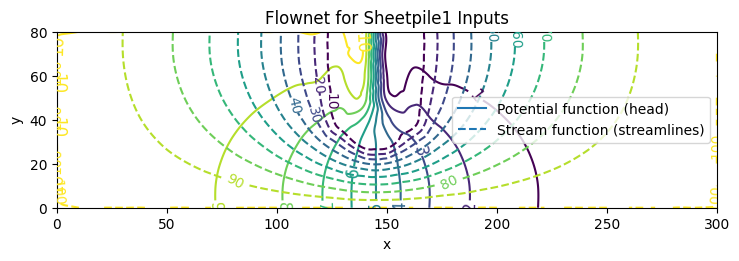
fig, ax = plot_flownet(
    "head_xyz.txt", "stream_xyz.txt",
    head_levels=[1,2,3,4,5,6,7,8,9,10],
    stream_levels=[10,20,30,40,50,60,70,80,90,100],
    title="Flownet for Sheetpile1 Inputs",
    save_png="flownet1.png",
    transparent=True
)

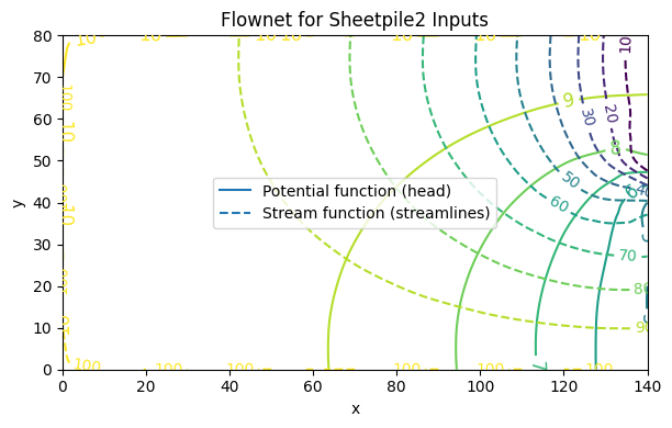
../../_images/4973ed9e42c8351386f7cd82fac3b50c465f9e1d4bef8c96be19bd7ac62c51d3.png

Flownet Example 2 : Pore Pressure under a Dam (Domain Decomposition approach)#

The second way to solve this example, and perhaps better is to take advantage of the symmetry and cut the domain in half, as

In this method we can actually specify the sheetpile as a boundary, and we will obtain the about same results, but only need to supply half as much input data.

Here’s the input file for the half-domain head calculations

10
10
1
9
15
1e-16
5000
10 20 30 40 50 60 70 80 90 100 110 120 130 140
70 60 50 40 30 20 10 0
1 1 1 1 1 1 1 1 1 1 1 1 1 1
0 0 0 0 0 0 0 0 0 0 0 0 0 0
1 1 1 1 1 1 1 1
0 0 0 1 1 1 1 1
10 10 10 10 10 10 10 10 10 10 10 10 10 10
10 10 10 10 10 10 10 10 10 10 10 10 10 10
10 10 10 10 10 10 10 10 10 10 10 10 10 10
10 10 10 10 10 10 10 10 10 10 10 10 10 10
10 10 10 10 10 10 10 10 10 10 10 10 10 5
10 10 10 10 10 10 10 10 10 10 10 10 10 5
10 10 10 10 10 10 10 10 10 10 10 10 10 5
10 10 10 10 10 10 10 10 10 10 10 10 10 5
10 10 10 10 10 10 10 10 10 10 10 10 10 5
0001 0.0001 0.0001 0.0001 0.0001 0.0001 0.0001 0.0001 0.0001 0.0001 0.0001 0.0001 0.0001 0.0001 0.0001
0001 0.0001 0.0001 0.0001 0.0001 0.0001 0.0001 0.0001 0.0001 0.0001 0.0001 0.0001 0.0001 0.0001 0.0001
0001 0.0001 0.0001 0.0001 0.0001 0.0001 0.0001 0.0001 0.0001 0.0001 0.0001 0.0001 0.0001 0.0001 0.0001
0001 0.0001 0.0001 0.0001 0.0001 0.0001 0.0001 0.0001 0.0001 0.0001 0.0001 0.0001 0.0001 0.0001 0.0001
0001 0.0001 0.0001 0.0001 0.0001 0.0001 0.0001 0.0001 0.0001 0.0001 0.0001 0.0001 0.0001 0.0001 0.0001
0001 0.0001 0.0001 0.0001 0.0001 0.0001 0.0001 0.0001 0.0001 0.0001 0.0001 0.0001 0.0001 0.0001 0.0001
0001 0.0001 0.0001 0.0001 0.0001 0.0001 0.0001 0.0001 0.0001 0.0001 0.0001 0.0001 0.0001 0.0001 0.0001
0001 0.0001 0.0001 0.0001 0.0001 0.0001 0.0001 0.0001 0.0001 0.0001 0.0001 0.0001 0.0001 0.0001 0.0001
0001 0.0001 0.0001 0.0001 0.0001 0.0001 0.0001 0.0001 0.0001 0.0001 0.0001 0.0001 0.0001 0.0001 0.0001
0001 0.0001 0.0001 0.0001 0.0001 0.0001 0.0001 0.0001 0.0001 0.0001 0.0001 0.0001 0.0001 0.0001 0.0001
0001 0.0001 0.0001 0.0001 0.0001 0.0001 0.0001 0.0001 0.0001 0.0001 0.0001 0.0001 0.0001 0.0001 0.0001
0001 0.0001 0.0001 0.0001 0.0001 0.0001 0.0001 0.0001 0.0001 0.0001 0.0001 0.0001 0.0001 0.0001 0.0001
0001 0.0001 0.0001 0.0001 0.0001 0.0001 0.0001 0.0001 0.0001 0.0001 0.0001 0.0001 0.0001 0.0001 0.0001
0001 0.0001 0.0001 0.0001 0.0001 0.0001 0.0001 0.0001 0.0001 0.0001 0.0001 0.0001 0.0001 0.0001 0.0001
0001 0.0001 0.0001 0.0001 0.0001 0.0001 0.0001 0.0001 0.0001 0.0001 0.0001 0.0001 0.0001 0.0001 0.0001
0001 0.0001 0.0001 0.0001 0.0001 0.0001 0.0001 0.0001 0.0001 0.0001 0.0001 0.0001 0.0001 0.0001 0.0001
0001 0.0001 0.0001 0.0001 0.0001 0.0001 0.0001 0.0001 0.0001 0.0001 0.0001 0.0001 0.0001 0.0001 0.0001
0001 0.0001 0.0001 0.0001 0.0001 0.0001 0.0001 0.0001 0.0001 0.0001 0.0001 0.0001 0.0001 0.0001 0.0001

%reset -f
from potential_flow_mod import read_potential_input, solve_potential
from flownet_plotter import write_xyz_grid, plot_flownet

# 1) Solve velocity potential (head)
modelp = read_potential_input("PotentialFnSheetpile2.txt")
head, niter, closure = solve_potential(modelp, verbose=False)
#fig = plot_head_contours(modelp.grid.distancex, modelp.grid.distancey, head, title="Contour Plot of Heads from Sheetpile1 Input")

# 2) Write solver outputs as XYZ (3 columns: x y value)
write_xyz_grid(modelp.grid.distancex, modelp.grid.distancey, head, "head_xyz.txt")

# 3) Solve stream function (streamlines)
models = read_potential_input("StreamFnSheetpile2.txt")
stream, niter, closure = solve_potential(models, verbose=False)
#fig = plot_head_contours(models.grid.distancex, models.grid.distancey, stream, title="Contour Plot of Heads from Sheetpile1 Input")

# 4) Write solver outputs as  XYZ (3 columns: x y value)
write_xyz_grid(models.grid.distancex, models.grid.distancey, stream, "stream_xyz.txt")

# 5) Make the flownet
fig, ax = plot_flownet(
    "head_xyz.txt", "stream_xyz.txt",
    head_levels=[1,2,3,4,5,6,7,8,9,10],
    stream_levels=[10,20,30,40,50,60,70,80,90,100],
    title="Flownet for Sheetpile2 Inputs",
    save_png="flownet2.png",
    transparent=True
)

../../_images/91708136e385cf6ece3eef318e969de4d923b7da31306694eee64976c31b45f0.png

Summary#

This chapter refreshed the governing equations of groundwater flow and the advection–dispersion equation for transport, emphasizing how Darcy’s law and mass conservation underpin both. Because you have seen these before, we focused on the essentials: storage terms (specific yield vs. specific storage), anisotropic conductivities, and how velocity fields from the flow solution drive transport. The aim was not to re-derive everything in full, but to recall the physics you need at your fingertips when you start building and checking models.

We then turned to flownets as a practical, low-overhead way to explore boundary effects and heterogeneity. Using a homebrew potential solver and flownet plotter, we showed how equipotential lines and stream functions can be overlaid to visualize flow patterns, estimate gradients, and even approximate capture zones—all without booting up MODFLOW. This approach is ideal for rapid “what-if” tests, classroom demonstrations, and early scoping on real sites. We noted anisotropy conceptually (directional conductivities) and left its detailed illustration as an exercise; extending the flownet to anisotropic cases is a natural next step. Together, these tools bridge theory and practice: they keep the physics honest while giving you fast, reproducible visuals that support interpretation and decision-making.

Exercise(s)#

Section End#

Back to top

3. Fundamentals (Practice)

Contents

3. Fundamentals (Practice)#

Scope#

Readings#

Videos#

Spreadsheets/Programs/Data#

Flow Equations#

Transport Equations#

Variables and constitutive pieces#

Species mass balance over a representative elementary volume (REV)#

Sorption and retardation (a type of reaction)#

(a) Instantaneous linear equilibrium sorption#

(b) Kinetic sorption (first-order two-rate; optional)#

(c) Dual-porosity / mobile–immobile (optional)#

Canonical forms (for direct use)#

Boundary conditions (quick reference)#

Units and sign checks#

Solving the Equations#

Flownets#

Example in Python#

Velocity Potential#

Stream Function#

Sheetpile under a dam flownet#

Flownet Example 2 : Pore Pressure under a Dam (Domain Decomposition approach)#

Summary#

Exercise(s)#

Section End#