8. Modeling Advection

8. Modeling Advection#

This section demonstrates advection modeling using two approaches: particle tracking and an upwind finite-difference scheme. These methods represent two distinct classes of simulation, chosen according to the needs of the problem. The underlying numerical-analysis details are covered in other courses. Note that advection is governed by hyperbolic PDEs, and effective solution techniques remain an active area of research.

Course Website

Link to Course Website

%%html
<style> table {margin-left: 0 !important;} </style>

Readings#

Videos#

Modeling advective transport in groundwater is a critical component of hydrogeology and environmental science, as it allows us to understand and predict the movement of contaminants and the transport of solutes through subsurface aquifers. Advective transport refers to the bulk movement of water and the substances it carries, driven primarily by hydraulic gradients and pressure differences within the groundwater system. This process plays a fundamental role in determining the fate and transport of pollutants, nutrients, and other substances in the subsurface environment.

A variety of widely used methods and techniques are used; These methodologies are essential for comprehending the dynamics of groundwater flow and the transport of substances within aquifers. Two popular methods for modeling advective transport in groundwater are numerical modeling and analytical solutions.

Numerical modeling stands as a cornerstone in the field, with models like MODFLOW (MODular Finite-Difference Ground-Water Flow Model) at the forefront. Numerical models divide the subsurface into discrete grid cells, considering various factors such as hydraulic conductivity, boundary conditions, and aquifer heterogeneity. These models utilize numerical algorithms to simulate the behavior of groundwater flow and contaminant transport over time. By incorporating data from field investigations, they enable scientists to make accurate predictions regarding the movement and fate of contaminants in complex geological settings. Numerical models are exceptionally versatile and can handle a wide range of scenarios, making them an indispensable tool for hydrogeologists and environmental scientists.

On the other hand, analytical solutions offer a more simplified approach for specific scenarios. These solutions are often employed when dealing with idealized geometries and boundary conditions. For instance, the advection-dispersion equation, a fundamental equation in groundwater transport, can be solved analytically for simple scenarios. Analytical solutions provide quick insights into transport phenomena and are valuable for initial assessments and educational purposes. However, they may not capture the complexities of real-world aquifers as effectively as numerical models.

Methods#

A reductionist point of view lets us categorize practical modeling methods into two categories: particle (parcel) tracking and eulerian finite- difference,element, or volume methods (marker-in-cell is a hybrid). The Eulerian methods almost always employ some kind of flux limiter to maintain proper mass balances, upwinding is one such approach. Particle tracking and upwind finite difference approaches are two distinct methods for modeling advective transport in groundwater, each with its own set of advantages and limitations. Let’s compare and contrast these approaches:

Particle Tracking:#

Conceptual Approach: Particle tracking models simulate the movement of individual particles within the groundwater flow field. This approach provides a more intuitive understanding of how contaminants or solutes move through the subsurface.
Accuracy in Complex Flow: Particle tracking is well-suited for modeling complex groundwater flow scenarios, such as in fractured aquifers or regions with varying flow directions. It can accurately represent irregular flow patterns.
Limitations: However, particle tracking may become computationally intensive when modeling a large number of particles over extended periods, making it less practical for long-term simulations.
Adaptive Resolution: It allows for adaptive grid refinement, where particles can be concentrated in regions of interest, offering higher resolution where needed.
Lagrangian Approach: It follows the Lagrangian approach, where particles move with the flow, which can be advantageous for understanding transport phenomena from a particle’s perspective.

Upwind Finite Difference:#

Grid-Based Approach: Upwind finite difference methods are grid-based, where the domain is divided into grid cells, and equations are solved at discrete locations within each cell.
Computational Efficiency: Upwind finite difference methods are computationally efficient for large-scale models and long-term simulations. They are widely used for regional-scale groundwater flow and transport modeling.
Stability: They are known for their numerical stability, which ensures that the solution remains accurate even when using relatively large time steps.
Accuracy in Uniform Flow: Upwind finite difference methods may perform very well in uniform flow conditions, but they can encounter challenges in accurately representing complex flow patterns, especially in situations where there are rapid changes in flow directions.
Eulerian Approach: These methods follow an Eulerian approach, where flow and transport equations are solved at fixed grid locations, making them less intuitive from a particle’s perspective.

In summary, the choice between particle tracking and upwind finite difference approaches for modeling advective transport in groundwater depends on the specific characteristics of the groundwater system and the research objectives:

Particle tracking is preferred for understanding transport at a detailed, particle-level scale and for modeling complex flow patterns.
Upwind finite difference methods are suitable for large-scale, long-term simulations where computational efficiency and stability are essential, especially in cases of relatively uniform flow.

Often, a combination of both methods may be employed in a modeling study to take advantage of their respective strengths, using particle tracking for detailed insights in specific areas and upwind finite difference methods for broader-scale simulations.

The remainder of this notebook presents simple examples of each method.

Note

While the methods in this notebook would be fine, practical “for money” modeling will usually employ specialized software; especially if lawyers will somehow get involved.

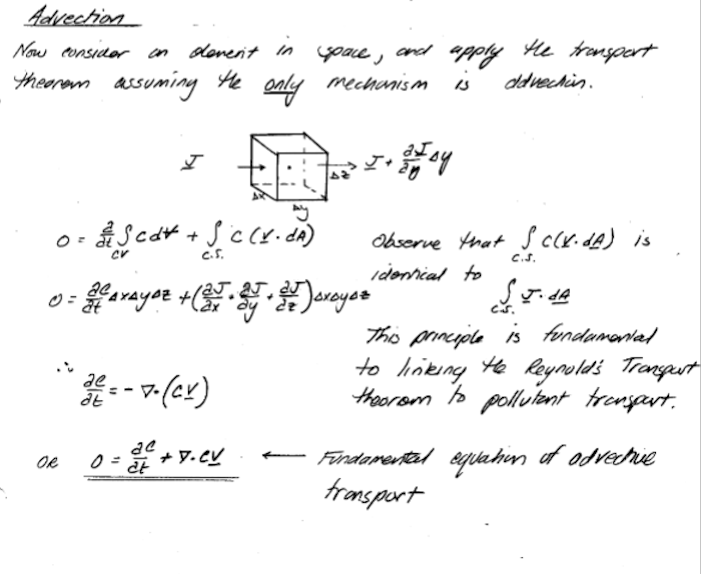
To build models, we simply apply the Reynolds Transport Theorem to the advective flux component to produce something like:

Modeling Advection by Particle Tracking (Lagrangian Approach)#

Later on we will use USGS-MOC (which incorporates particle tracking to define characteristic trajectories), so we will illustrate particle tracking keeping MOC in mind.

Particle or front tracking is typically performed using special software.
It can be performed using a spreadsheet.
The spreadsheet exercise is useful to illustrate the principles involved in particle tracking calculations.
Particle tracking with reactions is very computationally intensive and is beyond practical application in a spreadsheet; such computations are used to design space shuttles, helicopters and other things where the knowledge gained justifies the costs

The first step is to compute the velocity field (if it is steady even better, if not then every time increment it is recomputed)

If analytical functions are available for the velocity field then tracking is relatively easy.
Usually the velocity field is determined numerically at discrete points in space, and this is the situation of interest.
The interpolation schemes in common use are simple; simple, simple-linear, and multi-linear schemes.
Only the simple-linear scheme preserves cell-by-cell mass balances.

The figure below illustrates simple linear interpolation.

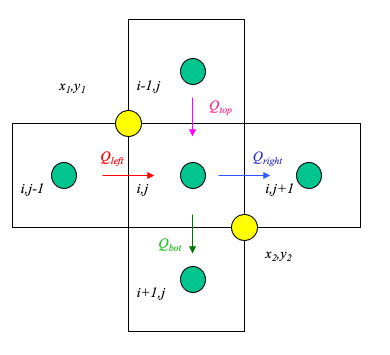
Typical computational grid for heads.
Arrows are the interfacial fluxes.
The simple scheme assigns the top and left flux to $(x_1,y_1)$.
The simple scheme assgins the right and bottom flux to $(x_2,y_2)$.

The particle velocity is determined by position of the particle relative to the velocity grid.

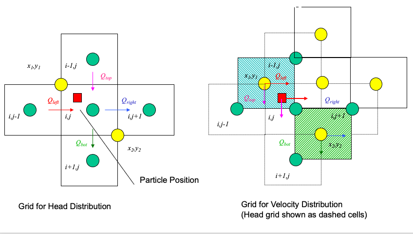
Uses the same grid as the head scheme. Velocity is the distance weighted average of the cell that the particle occupies.

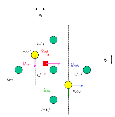
From the above figure, the particle’s velocities (x- and y- directions) are:

$u_p = \frac{1-\delta x}{\Delta x}u(x_1,y_1)+\frac{\delta x}{\Delta x}u(x_2,y_2)$
$v_p = \frac{1-\delta y}{\Delta y}v(x_1,y_1)+\frac{\delta y}{\Delta y}v(x_2,y_2)$

Multi-Linear Interpolation#

Higher order schemes produce smoother velocity fields at the expense of cell mass balances and computational ease. The USGS-MOC model uses a bi-linear scheme where the velocities at the four corners of the occupied cell are used. When transient flow fields occur, averaging in time is also used. The differences in the schemes are hard to detect when the grid spacing is small and the flow field is smoothly varying.

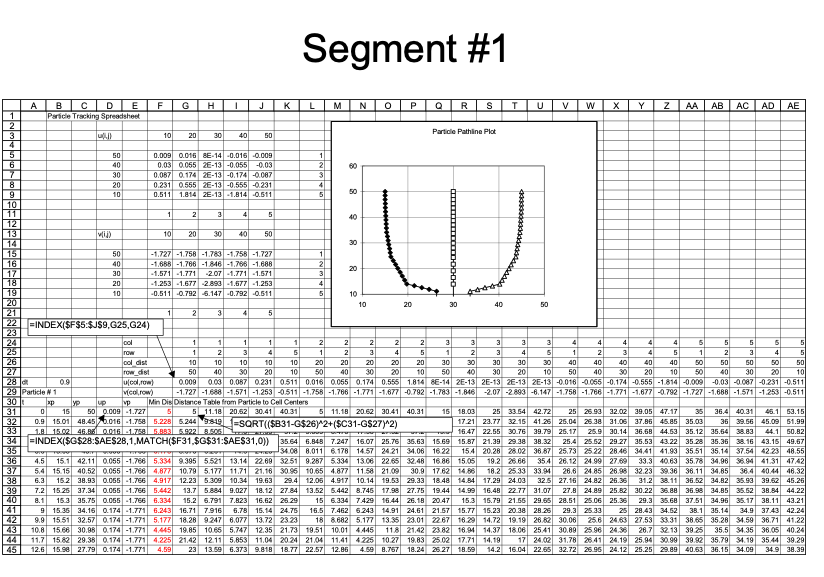
Spreadsheet (Excel) Approach#

To illustrate particle tracking the simple velocity scheme is used.
Extension to higher order schemes is straight forward.

Illustrate with simple scheme. Consider:

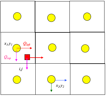
Large rectangles represent the velocity grid.
Circles represent the geometric location where velocity is known.
Small rectangle represents the particle that we wish to track.

Cell Indexing

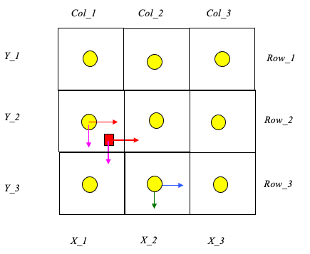
Each cell represents a grid location in the velocity field. Thus each cell has a unique row and column index.
Each cell centroid also has a unique geomteric (x,y) location.
The particle in the figure is located in cell named: Col_1,Row_2.
The cell is located at position: (X_1,Y_2).
The particle position is (XP,YP).

Locating the Particle

At the start of a time-step:
particle position is known.
cell positions are known.
cell that the particle occupies is unknown.
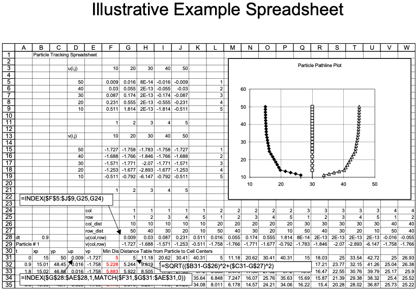
Construct a distance table
The distance from each cell to the particle is calculated and stored in a table.
Search the table,find the cell nearest the particle.
The cell coordinates of the smallest distance in the table is determined

Locating in Excel

The spreadsheet function that finds the value in an array (rectangular area of cells), given the position in the array to search is the function INDEX(array,row_index,column_index)
The spreadsheet function that can find the position in an array where a particular value appears is the function MATCH(value,array,type)

INDEX Function

INDEX(array,row_index,column_index) array is the location of the rectangular area of cells to search (eg. A3:C6). row_index is number of rows down from the starting row to search. column_index is the number of columns across from the starting column to search.

MATCH Function

MATCH(value,array,type) value is the numerical value to search for in the array. array is the location of the rectangular area of cells to search (eg. A3:C6). type is the type of match to use. type=0 means exact matching.

Using the Functions

The INDEX function allows us to select the correct values of velocity if we know which cell the particle resides in.
The MATCH function allows us to compare values in an array and determine the position in the array that these values are found.
Thus the MATCH function lets us search a distance table, find the cell center nearest the particle, and then use the index to find the correct velocity.

Moving the Particle

Once the cell containing the particle is identified, the particle is assigned the velocity values for that cell. The particle is then “moved” by the simple kinematic calculation:

$x_p(t+\Delta t)=x_p(t)+u_p(t)\Delta t$
$y_p(t+\Delta t)=y_p(t)+v_p(t)\Delta t$

Illustrative Example

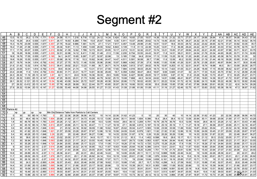
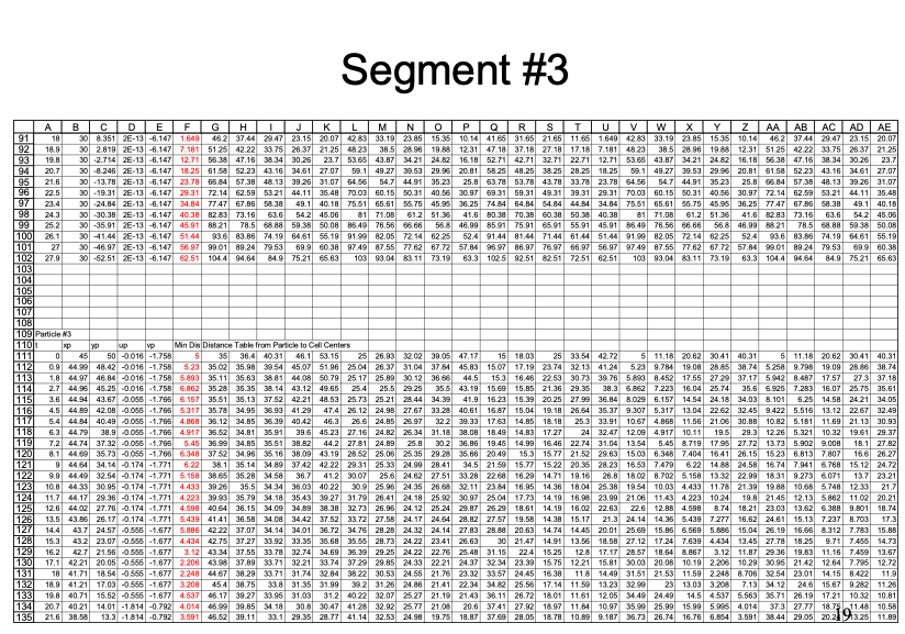
An example with 3 particles is shown below - the spreadsheet is kind of big because iterative computations are intentionally avoided.

Closer view for particle 1:

Closer view for particle 2:

Closer view for particle 3:

Summary

Particle tracking is a tool to determine the position of a fluid particle in a flow field.
A two-step approach is required:
Determine particle velocity
- Locate the particle relative to known velocity locations.
- Assign the velocity to the particle based on an interpolation scheme.
Move the particle.
All particle tracking programs use some sort of this two-step logic.
Extension to a 3rd spatial dimension is straightforward; boundaries are tricky - ray tracing and folding back across a boundary is a simple approach to manage a need to keep particles in a computational domain; alternatively

Spreadsheet Examples#

Tip

The 10X10 spreadsheet is known to work in LibreOffice (Open Source non-cloud based spreadsheet) as of 2025-0916

Performing the calculations in a python script is illustrated in the next section.

Note

You will see that the python script is simpler to construct than the spreadsheet (in terms of weird functions), but takes a shit-ton more code!

Particle Tracking in Python#

Here we illustrate using particle tracking to address a homework problem.

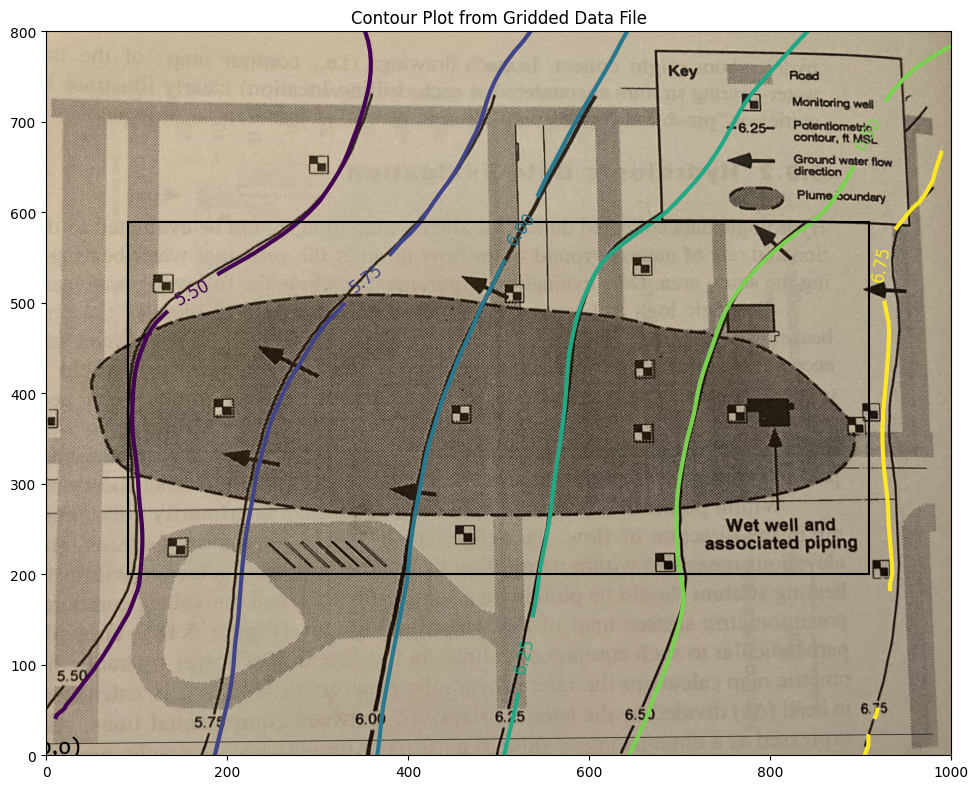
The figure below shows a piezometric map for a shallow sand aquifer. The hydraulic conductivtiy is estimated to be $1.5 \times 10^{-2}~\frac{cm}{s}$, the saturated thickness is 40 feet, and the effective porosity is 0.3.

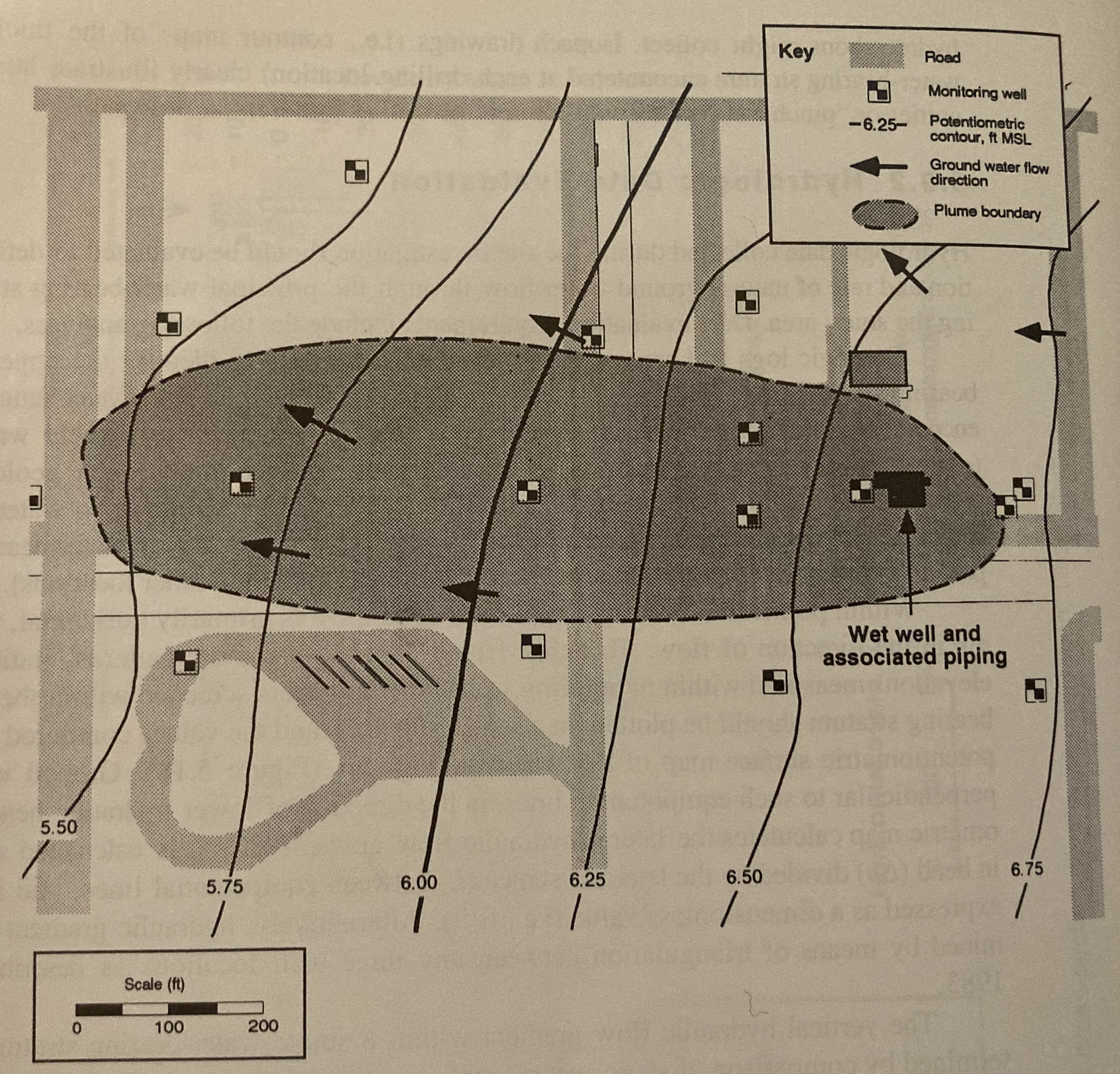
Determine:

Which well is expected to be the most contaminated.
The groundwater velocity and seepage velocity across the plume.
The duration that the source has been contaminating the aquifer (neglect dispersion, diffusiom, and adsorption).
The flow rate across the plume.
An explaination for contamination upgradient of the source zone.

Step 1. Need to Digitize the Head Map#

Use G3DATA or something similar to digitize the head map.

Step 2 Check the Digitization Results#

Here we will now produce a contour map from the digitized map, adjust sizes and overlay on the original map to get an idea of how good we did.

Also will use trial-and-error to find a useable hull within the contour plot where we can capture heads and use for a particle tracking effort - we have to find a rectangle with non-null interpolation values; easiest way (my opinion) is to try indices until can find a reasonable rectangle then sample from that rectangle. The process is documented below.

Note

The interpolation algorithm does not estimate vales outside the convex hull defined by the observation data. So the box below is by trial-and-error to stay within the convex hull; the interpolator in this region produces useable estimates for computing the heads and velocities from just the mapped information>

# CCMR from ENGR-1330:
# http://54.243.252.9/engr-1330-webroot/8-Labs/Lab07/Lab07.html
# https://clouds.eos.ubc.ca/~phil/docs/problem_solving/06-Plotting-with-Matplotlib/06.14-Contour-Plots.html
# https://docs.scipy.org/doc/scipy/reference/generated/scipy.interpolate.griddata.html
# https://stackoverflow.com/questions/332289/how-do-you-change-the-size-of-figures-drawn-with-matplotlib
# https://stackoverflow.com/questions/18730044/converting-two-lists-into-a-matrix
# https://stackoverflow.com/questions/3242382/interpolation-over-an-irregular-grid
# https://stackoverflow.com/questions/33919875/interpolate-irregular-3d-data-from-a-xyz-file-to-a-regular-grid
import pandas
my_xyz = pandas.read_csv('Fig5.18-LevelSets.png.dat',sep='\t') # read an ascii file already prepared, delimiter is tabs
#my_xyz = pandas.read_csv('XYZSomewhereUSA.txt',sep=' ') # read an ascii file already prepared, delimiter is tabs
my_xyz = pandas.DataFrame(my_xyz) # convert into a data frame
#print(my_xyz) #examine the dataframe
import numpy 
import matplotlib.pyplot
from scipy.interpolate import griddata
# extract lists from the dataframe
coord_x = my_xyz['X-Easting'].values.tolist()
coord_y = my_xyz['Y-Northing'].values.tolist()
coord_z = my_xyz['Z-Elevation'].values.tolist()
coord_xy = numpy.column_stack((coord_x, coord_y))
# Set plotting range in original data units
lon = numpy.linspace(min(coord_x), max(coord_x), 100)
lat = numpy.linspace(min(coord_y), max(coord_y), 100)
X, Y = numpy.meshgrid(lon, lat)
# Grid the data; use cubic spline interpolation (other choices are nearest and linear)
Z = griddata(numpy.array(coord_xy), numpy.array(coord_z), (X, Y), method='cubic', fill_value = 'nan')
# Build the map
print("Indices of black box on overlay below:")
ixl = 9
ixh = 90
iyl = 27
iyh = 62
print("xyz lower left corner ",X[iyl][ixl],Y[iyl][ixl],Z[iyl][ixl])
print("xyz lower right corner",X[iyl][ixh],Y[iyl][ixh],Z[iyl][ixh])
print("xyz upper left corner ",X[iyh][ixl],Y[iyh][ixl],Z[iyh][ixl])
print("xyz upper right corner ",X[iyh][ixh],Y[iyh][ixh],Z[iyh][ixh])
xxl = X[iyl][ixl]
xxh = X[iyh][ixh]
yyl = Y[iyl][ixl]
yyh = Y[iyh][ixh]
flag=True
if flag:
    matplotlib.pyplot.rcParams["figure.figsize"] = [10.00, 8.00]
    matplotlib.pyplot.rcParams["figure.autolayout"] = True
    im = matplotlib.pyplot.imread("Fig5.18-Coordinates.png") # base image
fig, ax = matplotlib.pyplot.subplots()
if flag: 
    im = ax.imshow(im, extent=[-25, 1000, -125, 800])# sets X and Y plot window of basemap
#fig.set_size_inches(14, 7)
levels=[5.50,5.75,6.00,6.25,6.50,6.75]
CS = ax.contour(X, Y, Z, levels, linewidths=3)
ax.clabel(CS, inline=2, fontsize=12)
ax.set_title('Contour Plot from Gridded Data File')
ax.set_xlim([0,1000])
ax.set_ylim([0,800])
ax.plot([xxl,xxh],[yyl,yyl],color="black")
ax.plot([xxl,xxh],[yyh,yyh],color="black")
ax.plot([xxl,xxl],[yyl,yyh],color="black")
ax.plot([xxh,xxh],[yyl,yyh],color="black");

Indices of black box on overlay below:
xyz lower left corner  90.9090909090909 200.0 5.478952367771485
xyz lower right corner 909.090909090909 200.0 6.7224489855441645
xyz upper left corner  90.9090909090909 588.8888888888889 5.302942021834025
xyz upper right corner  909.090909090909 588.8888888888889 6.663235234576626

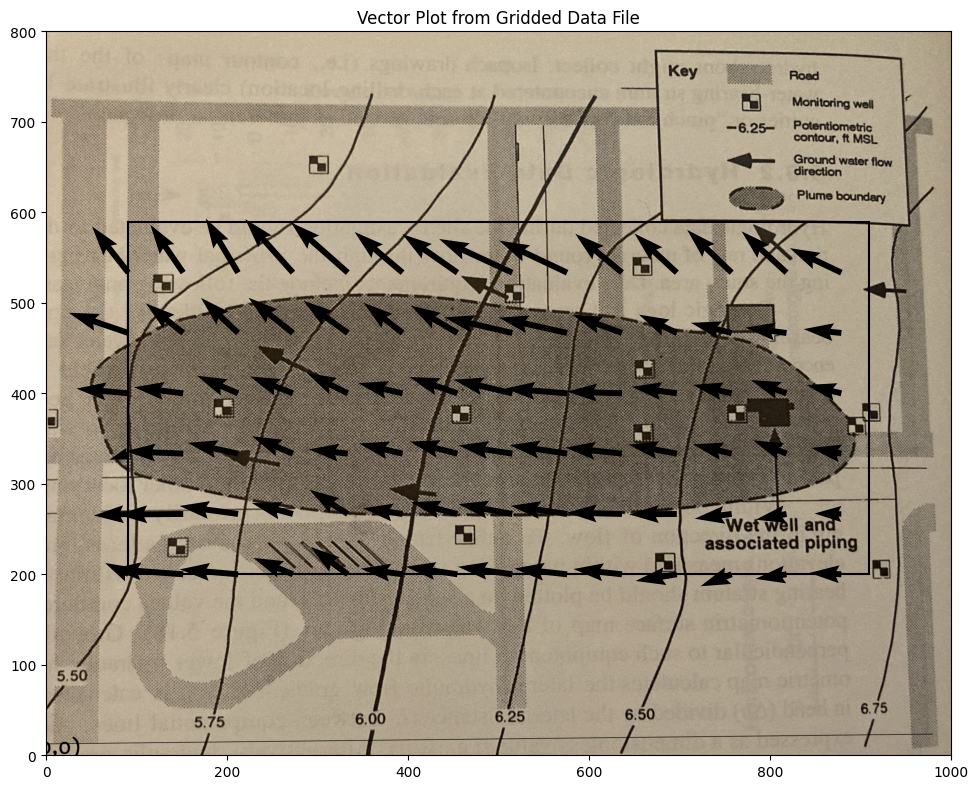
../../_images/1a9f6dda9e0b4aa1354015bd7bbc4da23c85c4d26106035c451571e0528dbbda.png

This is acceptable. Now we will extract velocities from the gridded data files - using the “box”. Recall to use the spreadsheet version of the particle tracker we need the $U$ and $V$ fields from the head distribution.

We will use the supplied hydraulic conductivity and porosity

$K~\approx~ 1.5 \times 10^{-2}~\frac{cm}{s} \cdot \frac{1~in}{2.54~cm} \cdot \frac{1~ft}{12~in} \cdot \frac{86400~s}{1~day} = 42.52~\frac{ft}{day}$
$n~\approx~ 0.30 $

And apply Darcy’s law as

$\textbf{u(x,y)} = -\frac{K}{n}\cdot \frac{\Delta h}{\Delta x}$
$\textbf{v(x,y)} = -\frac{K}{n}\cdot \frac{\Delta h}{\Delta y}$

Conductivity = 42.52 # feet/day
Porosity = 0.30 # voids/bulk
nrows = iyh - iyl
ncols = ixh - ixl
#Zero vectors for the velocity fields
U = [[0 for j in range(ncols)] for i in range(nrows)]
V = [[0 for j in range(ncols)] for i in range(nrows)]
#Zero vectors for realinged mesh grid
XG = [[0 for j in range(ncols)] for i in range(nrows)]
YG = [[0 for j in range(ncols)] for i in range(nrows)]
for j in range(ncols):
    for i in range(nrows): #range(nrows)
        U[i][j] = -1.0*(Conductivity/Porosity)*(Z[iyl+i][ixl+j]-Z[iyl+i][ixl+j-1])/(X[iyl+i][ixl+j]-X[iyl+i][ixl+j-1]) #- K dh/dx
        V[i][j] = -1.0*(Conductivity/Porosity)*(Z[iyl+i][ixl+j]-Z[iyl+i-1][ixl+j])/(Y[iyl+i][ixl+j]-Y[iyl+i-1][ixl+j]) #- K dh/dy
        XG[i][j] = X[iyl+i][ixl+j]
        YG[i][j] = Y[iyl+i][ixl+j]

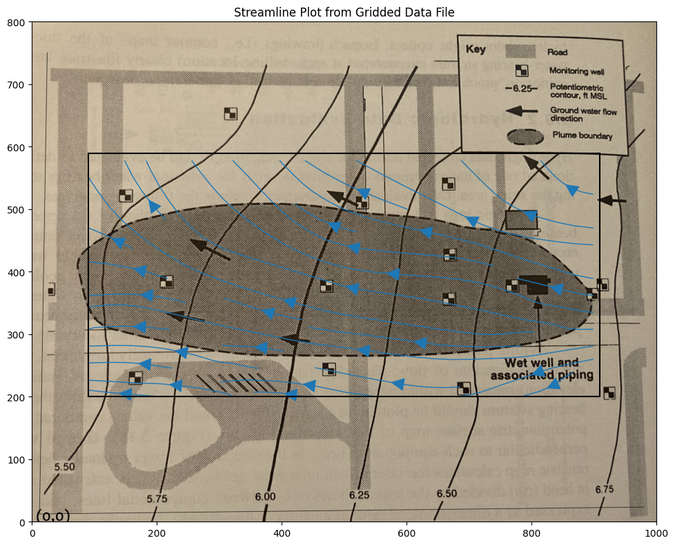
Suppose we want a plot of the vector field just to check our work, a nice tool is quiver and/or streamplot which are demonstrated below

# convert to numpy arrays
UU = numpy.asarray(U)
VV = numpy.asarray(V)
XX = numpy.asarray(XG)
YY = numpy.asarray(YG)

UU[30][30]

np.float64(-0.2250452891747141)

Now a cool “quiver” plot

if flag:
    matplotlib.pyplot.rcParams["figure.figsize"] = [10.00, 8.00]
    matplotlib.pyplot.rcParams["figure.autolayout"] = True
    im = matplotlib.pyplot.imread("Fig5.18-Coordinates.png") # base image
fig, ax = matplotlib.pyplot.subplots()
if flag: 
    im = ax.imshow(im, extent=[-25, 1000, -125, 800])# sets X and Y plot window of basemap
#fig.set_size_inches(14, 7)
levels=[5.50,5.75,6.00,6.25,6.50,6.75]
CS = ax.quiver(XX[::6, ::6], YY[::6, ::6], UU[::6, ::6], VV[::6, ::6], units='width')
#ax.clabel(CS, inline=2, fontsize=12)
ax.set_title('Vector Plot from Gridded Data File')
ax.set_xlim([0,1000])
ax.set_ylim([0,800]);
ax.plot([xxl,xxh],[yyl,yyl],color="black")
ax.plot([xxl,xxh],[yyh,yyh],color="black")
ax.plot([xxl,xxl],[yyl,yyh],color="black")
ax.plot([xxh,xxh],[yyl,yyh],color="black");

#matplotlib.pyplot.quiver(XX[::6, ::6], YY[::6, ::6], UU[::6, ::6], VV[::6, ::6], units='width')
#matplotlib.pyplot.streamplot(XX, YY, UU, VV, density=0.5, linewidth=2, color=None)

../../_images/8367502528ff7611e622a7cd79e76576fc5b3ff90bb1824f2b51e8dba9656e79.png

if flag:
    matplotlib.pyplot.rcParams["figure.figsize"] = [10.00, 8.00]
    matplotlib.pyplot.rcParams["figure.autolayout"] = True
    im = matplotlib.pyplot.imread("Fig5.18-Coordinates.png") # base image
fig, ax = matplotlib.pyplot.subplots()
if flag: 
    im = ax.imshow(im, extent=[0, 1000, -125, 800])# sets X and Y plot window of basemap
#fig.set_size_inches(14, 7)
levels=[5.50,5.75,6.00,6.25,6.50,6.75]
CS = ax.streamplot(XX, YY, UU, VV,  density=0.5, linewidth=1, color=None, arrowsize=3)
#ax.clabel(CS, inline=2, fontsize=12)
ax.set_title('Streamline Plot from Gridded Data File')
ax.set_xlim([0,1000])
ax.set_ylim([0,800]);
ax.plot([xxl,xxh],[yyl,yyl],color="black")
ax.plot([xxl,xxh],[yyh,yyh],color="black")
ax.plot([xxl,xxl],[yyl,yyh],color="black")
ax.plot([xxh,xxh],[yyl,yyh],color="black");

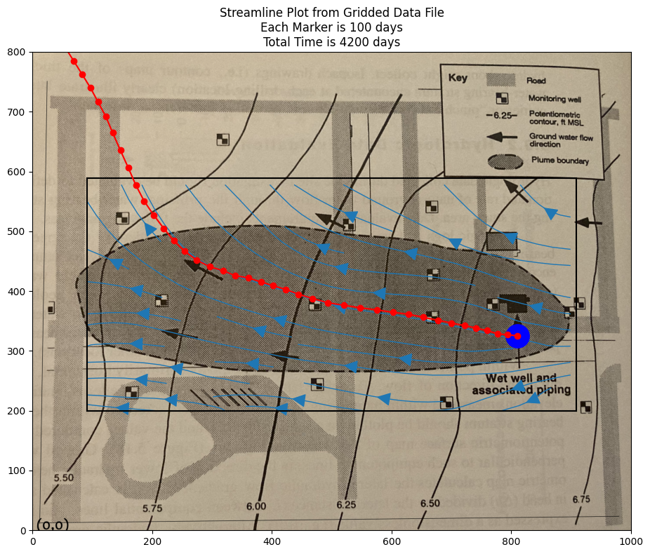
../../_images/a42eea28397e1d380365e9c5008f6a5286321114971bf84d4610604249875b13.png

Now we can implement a particle tracking script. Using the spreadsheet as a guide we can write it in python, and access the cool graphics.

Here is the basic script, one simply has to wrap it into a time-stepping loop to produce a trajectory. Multiple particles can be managed

# U array x-velocity at XG,YG
# V array y-velocity at XG,YG
# XG array X-value of cell center
# YG array Y-value of cell center
# XP X-value of particle position 
# YP Y-value of particle position
# UP x-velocity of particle 
# VP y-velocity of particle
# TX x-component particle trajectory
# TY y-component particle trajectory

import math
verbose=False
terse=False
deltaT = 100
etime = 0
numTime = 42
XP = []
YP = []
UP = []
VP = []
TX = [] #trajectory vector
TY = []
np = 1 # Total particles 
XP.append(825)
YP.append(325)
UP.append(0)
VP.append(0)
ip=np-1 
print("                   Initial Particle Position",round(XP[ip],2),round(YP[ip],2),round(UP[ip],2),round(VP[ip],2),round(etime,2))

# move particles this time step
for it in range(numTime):
    for ip in range(np):
    # Build Particle Distance Table
        dist = []
        index = []
        count = 0
        for j in range(ncols):
            for i in range(nrows): #range(nrows)
                dist.append(math.sqrt((XX[i][j]-XP[ip])**2 + (YY[i][j]-YP[ip])**2))
                index.append([count,i,j]) # use to find i,j for a given index
                count = count +1
    # find closest cell
        for i in range(count):
            if dist[i] <= min(dist):
                #print(index[i],dist[i])
                ixx=index[i][1]
                jyy=index[i][2]
    # use nearest cell assignment - aka simple scheme
                UP[ip] = UU[ixx][jyy]
                VP[ip] = VV[ixx][jyy]
                if verbose: print("Particle Position and Velocities Before Move",round(XP[ip],2),round(YP[ip],2),round(UP[ip],2),round(VP[ip],2),round(etime,2))
                break #exits the loop - we stop at the first nearest cell encountered
    # move the particle
        XP[ip]=XP[ip]+UP[ip]*deltaT
        YP[ip]=YP[ip]+VP[ip]*deltaT
        etime=etime+deltaT
        if terse: print(" Particle Position and Velocities After Move",round(XP[ip],2),round(YP[ip],2),round(UP[ip],2),round(VP[ip],2),round(etime,2))
        TX.append([ip,XP[ip],etime])
        TY.append([ip,YP[ip],etime])

                   Initial Particle Position 825 325 0 0 0

if flag:
    matplotlib.pyplot.rcParams["figure.figsize"] = [10.00, 8.00]
    matplotlib.pyplot.rcParams["figure.autolayout"] = True
    im = matplotlib.pyplot.imread("Fig5.18-Coordinates.png") # base image
fig, ax = matplotlib.pyplot.subplots()
if flag: 
    im = ax.imshow(im, extent=[0, 1000, -125, 800])# sets X and Y plot window of basemap
#fig.set_size_inches(14, 7)
levels=[5.50,5.75,6.00,6.25,6.50,6.75]
CS = ax.streamplot(XX, YY, UU, VV,  density=0.5, linewidth=1, color=None, arrowsize=3)
#ax.clabel(CS, inline=2, fontsize=12)
ax.set_title('Streamline Plot from Gridded Data File\n' +\
            'Each Marker is ' + str(deltaT) + ' days\n' +\
            'Total Time is ' + str(etime) + ' days')
ax.set_xlim([0,1000])
ax.set_ylim([0,800]);
ax.plot([xxl,xxh],[yyl,yyl],color="black")
ax.plot([xxl,xxh],[yyh,yyh],color="black")
ax.plot([xxl,xxl],[yyl,yyh],color="black")
ax.plot([xxh,xxh],[yyl,yyh],color="black")
xtrajectory = [sublist[1] for sublist in TX]
ytrajectory = [sublist[1] for sublist in TY]
ax.plot(xtrajectory[0],ytrajectory[0],marker="o",color="blue",markersize=24)
ax.plot(xtrajectory,ytrajectory,marker="o",color="red")
;

''

../../_images/bbae6304d363b7919857c128f6777543b034a3cd5a2023445fa1f50c40943b1c.png

Extensions#

One could certainly add a lot more particles.
If the parcels represent some quantify of mass, concentrations can be directly approximated.

The method is not limited to groundwater hydrology, it is useful for surface water hydrology to find flow paths for time-of-concentration calculations; extension to the 3rd spatial dimension is also straightforward.

Modeling Advection by Finite-Difference (Eulerian Approach)#

The transport equations are partial differential equations (PDEs), which describe the evolution of a quantity over space and time. One of the most common methods for solving these equations numerically is the finite-difference method (FDM). This approach discretizes space and time into a grid and approximates the derivatives of the governing equations.

Finite-Difference Method#

In the finite-difference method, spatial and temporal domains are discretized into small steps. The derivatives in the governing transport PDE are approximated using the differences between neighboring grid points.

For example, consider the 1D advection equation (a typical transport equation): $$\frac{\partial C}{\partial t} = - V \frac{\partial C}{\partial x}$$

where $C(x,t)$ is the transported quantity (e.g., concentration), $V$ is the advection velocity, and $t$ and $x$ are time and space, respectively.

To solve approximate the solution using finite-difference, we could approximate the derivatives as:

\[\frac{\partial C}{\partial t} \approx \frac{C_i^{n+1} - C_i^n}{\Delta t}~\text{(time derivative, forward difference)}\]

\[\frac{\partial C}{\partial x} \approx \frac{C_{i+1}^{n} - C_{i-1}^n}{2 \Delta x}~\text{(spatial derivative, centered difference)}\]

However, the simple central difference approximation for the spatial derivative may lead to non-physical oscillations or instability, particularly when solving hyperbolic dominanted transport equations like the advection equation.

Upwinding in Hyperbolic-Dominant PDEs#

In transport modeling, hyperbolic PDEs (like the advection equation) describe wave propagation and are characterized by the dominance of the advection term. When solving such equations numerically, the choice of difference scheme is critical for stability and accuracy.

Upwind differencing is a technique specifically designed to handle hyperbolic PDEs. The idea is to use information from the direction of the flow (upstream) to approximate the spatial derivative. This prevents the introduction of non-physical oscillations by ensuring that the finite-difference scheme respects the direction of the characteristic waves (i.e., the direction in which information propagates). Upwind Scheme

For a simple 1D advection equation, if the flow velocity $V>0$ (information travels to the right), we use the backward difference to approximate the spatial derivative: $$\frac{\partial C}{\partial x} \approx \frac{C_{i}^{n} - C_{i-1}^n}{\Delta x}~\text{(spatial derivative, backward difference)}$$

If $V<0$ (information travels to the left), we use the forward difference:

\[\frac{\partial C}{\partial x} \approx \frac{C_{i+1}^{n} - C_{i}^n}{\Delta x}~\text{(spatial derivative, forward difference)}\]

This technique, called upwinding, introduces numerical dissipation that stabilizes the solution and prevents oscillations, but it does so at the cost of some accuracy (it can be less accurate for smooth solutions compared to central differencing).

Why Upwinding is Important#

Upwinding is essential in transport modeling because most real-world problems involve advection-dominated transport, where sharp fronts or discontinuities are common (e.g., contaminant plumes or shock waves). Without upwinding, traditional finite-difference methods can result in:

Non-physical oscillations: especially when trying to capture sharp gradients.
Instability: numerical solutions can blow up if the scheme is not carefully designed for hyperbolic systems.
Artificial diffusion: even stable solutions will have apparent added diffusion that is absent from the physical system.

By incorporating upwinding, we align the numerical method with the physics of the problem, ensuring that information propagates in the correct direction, thereby stabilizing the simulation.

A simple example follows to illustrate the effect of upwinding and no upwinding.

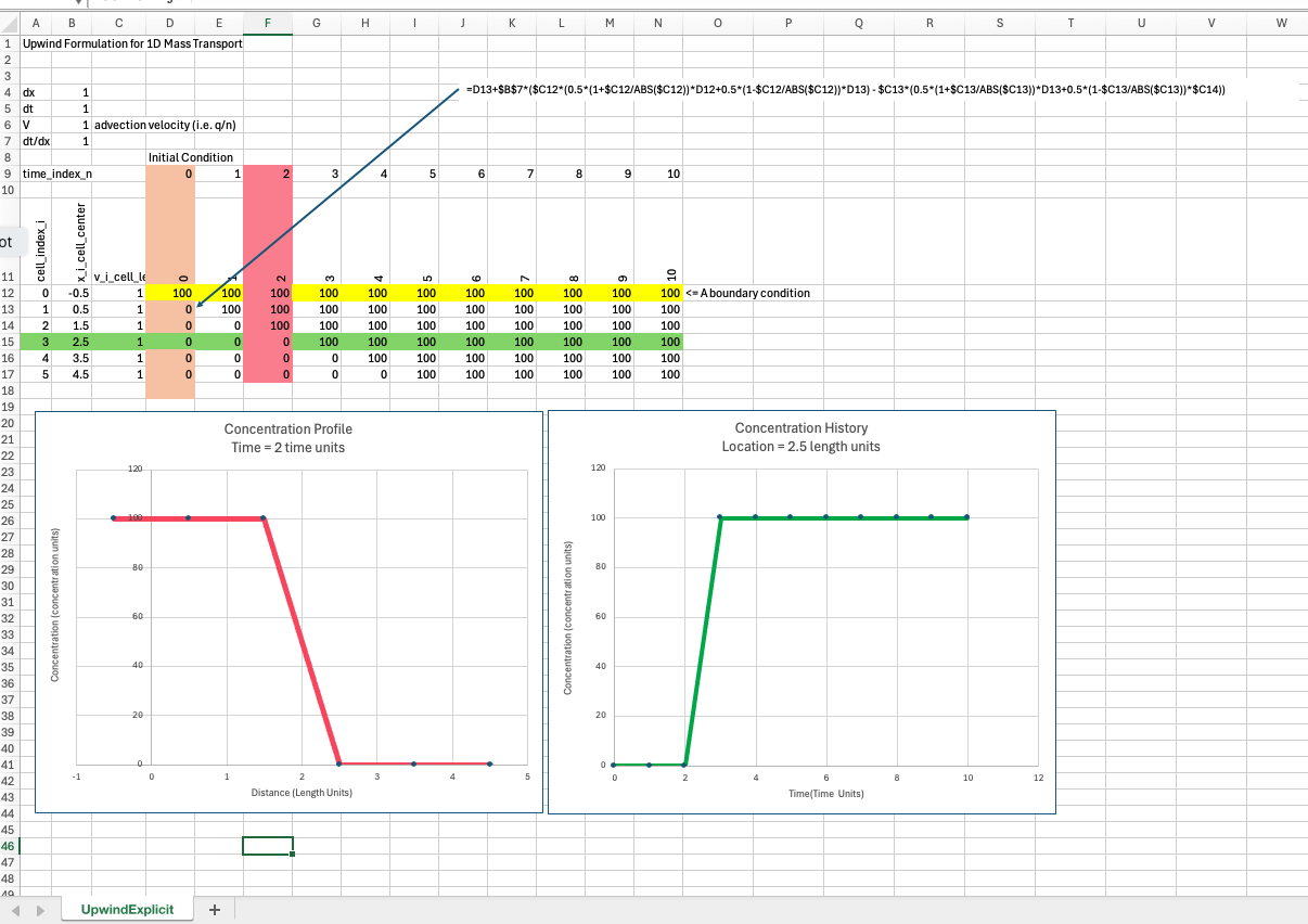
Upwind formulation#

A simple upwind formulation for 1D system is

\[C_i^{n+1} = C_i^n + \frac{\Delta t}{\Delta x}(V_{i-1}[\frac{1}{2}(1+\frac{V_{i-1}}{|V_{i-1}|})C_{i-1}^{n}+\frac{1}{2}(1-\frac{V_{i-1}}{|V_{i-1}|})C_{i}^{n}]-V_{i}[\frac{1}{2}(1+\frac{V_{i}}{|V_{i}|})C_{i}^{n}+\frac{1}{2}(1-\frac{V_{i}}{|V_{i}|})C_{i+1}^{n}])\]

The parts with the absolute value are a sneaky way to handle the upwinding automatically.

As long as $V_i <= \frac{\Delta t}{\Delta x}$ this difference scheme is stable, it is also reasonably accurate if $V_i \approx \frac{\Delta t}{\Delta x}$

Below is a simple spreadsheet implementation of the explicit scheme above.

In MODFLOW6 transport model, a choice of upwind (called upstream in the toolkit) tries to match internal time steps to maintain numerical stability. As you will see in class when we run a spreadsheet example. Its impossible for perfect accuracy and stability, but it is possible to stay close. We will see examples of numerical diffusion as we depart from the accuracy requirement.

Below is a flexible NumPy framework for 1-D upwind (Godunov) advection updating. It implements a flux-splitting form that’s algebraically equivalent to the simple upwind formulation but avoids division by zero when $V=0$.

The code below uses the equivalent flux-splitting form where the cell interface fluxes are computed as:

$F_{i+1/2}=max(V_i,0) \cdot C_i + min(V_i,0) \cdot C_{i+1}$

and the resulting mass balance is:

$C_i^{n+1}=C_i^n +\frac{\Delta t}{\Delta x}(F_{i−1/2}−F_{i+1/2})$.

import numpy as np

def upwind_1d(
    C0: np.ndarray,
    v,                     # scalar, (nx,), (nt,), or (nt, nx)
    dx: float,
    dt: float,
    nt: int,
    C_left=None,           # left Dirichlet BC: scalar or array length nt+1/nt
    C_right=None           # right Dirichlet BC: scalar or array length nt+1/nt
) -> np.ndarray:
    """
    First-order upwind finite-difference solver for 1D advection:
        C_i^{n+1} = C_i^n + (dt/dx) * (F_{i-1/2} - F_{i+1/2})
    with interface flux (Godunov/flux-splitting):
        F_{i+1/2} = max(v_i,0)*C_i + min(v_i,0)*C_{i+1}

    Parameters
    ----------
    C0 : (nx,) array
        Initial concentration profile at t=0.
    v : scalar | (nx,) | (nt,) | (nt,nx)
        Velocity. Interpreted at cell interfaces i = 0..nx-2 as v[i].
        - scalar: constant in space & time
        - (nx,): spatially varying, constant in time
        - (nt,): time-varying, uniform in space
        - (nt,nx): varying in space & time (uses v[n, i] at interfaces)
    dx, dt : float
        Grid spacing and time step.
    nt : int
        Number of time steps to advance.
    C_left, C_right : scalar | array | None
        Dirichlet boundary concentration at x=0 and x=L.
        If array, may be length nt or nt+1; if scalar, held constant.
        If None, defaults:
            - left: hold C[0] fixed at its initial value
            - right: zero-gradient outflow (C[-1] = C[-2] each step)

    Returns
    -------
    C : (nt+1, nx) array
        Concentration field over time (including the initial state).
    """
    C0 = np.asarray(C0, dtype=float)
    nx = C0.size
    if nx < 2:
        raise ValueError("C0 must have length >= 2.")

    # --- Broadcast velocity to shape (nt, nx) for convenience ---
    v_arr = _broadcast_velocity(v, nt, nx)

    # --- Prepare boundary series ---
    left_series  = _expand_bc(C_left,  nt, default=C0[0])
    right_series = _expand_bc(C_right, nt, default=None)  # None => outflow

    # --- CFL check (conservative, using max over provided v) ---
    vmax = np.nanmax(np.abs(v_arr))
    if vmax > 0 and (dt/dx) * vmax > 1.0 + 1e-12:
        print(f"⚠️ CFL warning: (dt/dx)*max|v| = {(dt/dx)*vmax:.3f} > 1. "
              "First-order upwind may become unstable. Consider reducing dt.")

    # --- Allocate solution ---
    C = np.zeros((nt+1, nx), dtype=float)
    C[0] = C0

    for n in range(nt):
        # Apply/hold left Dirichlet at time level n before fluxes
        C[n, 0] = left_series[n]  # if left_series is default, this holds C[0] fixed

        # Velocity at interfaces for this step: use first nx-1 entries
        v_n = v_arr[n, :]

        # Interface fluxes between i and i+1 for i = 0..nx-2
        # F[i] = flux through the interface between cell i and cell i+1
        F = np.maximum(v_n[:-1], 0.0) * C[n, :-1] + np.minimum(v_n[:-1], 0.0) * C[n, 1:]

        # Update interior cells i = 1..nx-2
        C[n+1, 1:-1] = C[n, 1:-1] + (dt/dx) * (F[:-1] - F[1:])

        # Left boundary (Dirichlet at next time)
        C[n+1, 0] = left_series[n+1]

        # Right boundary
        if right_series is None:
            # Zero-gradient (advective outflow): copy neighbor after update
            C[n+1, -1] = C[n+1, -2]
        else:
            # Dirichlet at the right boundary
            C[n+1, -1] = right_series[n+1]

    return C


# ---------- Helpers ----------

def _broadcast_velocity(v, nt, nx):
    """
    Return velocity array of shape (nt, nx).
    Interprets v[..., i] as the velocity used at interface i (between i and i+1).
    The last column (i = nx-1) is unused and may be ignored, but we keep shape uniform.
    """
    if np.isscalar(v):
        v_arr = np.full((nt, nx), float(v))
    else:
        v = np.asarray(v, dtype=float)
        if v.ndim == 1:
            if v.size == nx:
                v_arr = np.repeat(v[np.newaxis, :], nt, axis=0)
            elif v.size == nt:
                v_arr = np.repeat(v[:, np.newaxis], nx, axis=1)
            else:
                raise ValueError("v length must be nx or nt if 1D.")
        elif v.ndim == 2:
            if v.shape != (nt, nx):
                raise ValueError(f"v shape must be (nt, nx) if 2D; got {v.shape}.")
            v_arr = v
        else:
            raise ValueError("v must be scalar, 1D, or 2D.")
    return v_arr


def _expand_bc(bc, nt, default=None):
    """
    Normalize boundary condition to a series of length nt+1.
    - If bc is None: returns default behavior
        * left: return an array that repeats default (Dirichlet hold)
        * right: returns None to signal outflow handling
    - If scalar: constant BC over time
    - If array-like length nt or nt+1: broadcast to length nt+1
    """
    if bc is None:
        # left: use default value; right: signal open boundary with None
        return None if default is None else np.full(nt+1, float(default))

    if np.isscalar(bc):
        return np.full(nt+1, float(bc))

    bc = np.asarray(bc, dtype=float).ravel()
    if bc.size == nt:
        # Extend by repeating the last value
        return np.concatenate([bc, bc[-1:]])
    if bc.size == nt + 1:
        return bc

    raise ValueError("Boundary series must be scalar or length nt or nt+1.")

import numpy as np
import matplotlib.pyplot as plt

def plot_profiles(C, x, times, dt, ax=None, title="Profiles at selected times"):
    """
    Plot C(x, t) for several physical times.

    Parameters
    ----------
    C : array, shape (nt+1, nx)
        Solution including initial condition at t=0.
    x : array, shape (nx,)
        Grid coordinates.
    times : list/array of floats
        Physical times to plot (same units as dt).
    dt : float
        Time step size.
    ax : matplotlib.axes.Axes or None
        Optional axis to draw on. Creates one if None.
    title : str
        Plot title.

    Returns
    -------
    ax : matplotlib.axes.Axes
    used_times : ndarray of floats
        The actual times used (snapped to the time grid).
    used_indices : ndarray of ints
        The corresponding time indices.
    """
    C = np.asarray(C); x = np.asarray(x)
    nt = C.shape[0] - 1

    # Map requested times to nearest indices
    k_list, t_used = [], []
    for t in np.atleast_1d(times):
        k = int(round(t / dt))
        k = max(0, min(nt, k))
        k_list.append(k)
        t_used.append(k * dt)
    k_list = np.array(k_list, dtype=int)
    t_used = np.array(t_used, dtype=float)

    if ax is None:
        fig, ax = plt.subplots(figsize=(8, 4.5))

    for k, tval in zip(k_list, t_used):
        ax.plot(x, C[k, :], label=f"t = {tval:.3g}")

    ax.set_xlabel("x")
    ax.set_ylabel("C")
    ax.set_title(title)
    ax.grid(True, alpha=0.3)
    ax.legend()
    plt.tight_layout()
    return ax, t_used, k_list


def plot_histories(C, x, x_locs, dt, ax=None, by="coord", title="Concentration Histories at selected locations"):
    """
    Plot C(t) at several spatial locations.

    Parameters
    ----------
    C : array, shape (nt+1, nx)
        Solution including initial condition at t=0.
    x : array, shape (nx,)
        Grid coordinates.
    x_locs : list/array
        If by='coord': physical x-locations to sample (floats).
        If by='index': integer node indices.
    dt : float
        Time step size.
    ax : matplotlib.axes.Axes or None
        Optional axis to draw on. Creates one if None.
    by : {'coord','index'}
        How to interpret x_locs.
    title : str
        Plot title.

    Returns
    -------
    ax : matplotlib.axes.Axes
    used_indices : ndarray of ints
        Grid indices actually plotted.
    """
    C = np.asarray(C); x = np.asarray(x)
    nt, nx = C.shape[0]-1, C.shape[1]
    t = np.arange(nt+1) * dt

    # Map requested locations to indices
    j_list = []
    if by == "coord":
        for x0 in np.atleast_1d(x_locs):
            j = int(np.argmin(np.abs(x - float(x0))))
            j_list.append(j)
    elif by == "index":
        for j in np.atleast_1d(x_locs):
            j_list.append(int(np.clip(int(j), 0, nx-1)))
    else:
        raise ValueError("by must be 'coord' or 'index'.")

    j_list = np.array(j_list, dtype=int)

    if ax is None:
        fig, ax = plt.subplots(figsize=(8, 4.5))

    for j in j_list:
        ax.plot(t, C[:, j], label=f"x ≈ {x[j]:.3g} (j={j})")

    ax.set_xlabel("t")
    ax.set_ylabel("C")
    ax.set_title(title)
    ax.grid(True, alpha=0.3)
    ax.legend()
    plt.tight_layout()
    return ax, j_list

import numpy as np

def rectangular_pulse_centered(x, x0, width, C0=1.0):
    """
    Node-based top-hat: C(x) = C0 for |x - x0| <= width/2, else 0.
    """
    x = np.asarray(x)
    half = 0.5 * float(width)
    return C0 * ((x >= x0 - half) & (x <= x0 + half)).astype(float)

def rectangular_pulse_segment(x, x1, x2, C0=1.0):
    """
    Node-based top-hat: C(x) = C0 for x1 <= x <= x2, else 0.
    """
    x = np.asarray(x)
    lo, hi = min(x1, x2), max(x1, x2)
    return C0 * ((x >= lo) & (x <= hi)).astype(float)

def rectangular_pulse_cellavg(x, dx, x1, x2, C0=1.0):
    """
    Cell-averaged top-hat for uniform grid with centers at x and spacing dx.
    For each cell, compute overlap length with [x1, x2] and scale by C0*(overlap/dx).
    """
    x = np.asarray(x, dtype=float)
    lo, hi = min(x1, x2), max(x1, x2)
    left_edges  = x - 0.5*dx
    right_edges = x + 0.5*dx
    overlap = np.maximum(0.0, np.minimum(right_edges, hi) - np.maximum(left_edges, lo))
    return C0 * (overlap / dx)

# Grid
nx = 201
x = np.linspace(0.0, 1.0, nx)
dx = x[1] - x[0]

# Gaussian pulse centered at x0 with sd w and height C0
x0, w, C0 = 0.2, 0.025, 100.0
C_init = C0*np.exp(-((x - x0)/w)**2)   
# Rectangular pulse centered at x0 with width w and height C0
#x0, w, C0 = 0.05, 0.10, 0.0
# Option A: node-based
#C_init = rectangular_pulse_centered(x, x0, w, C0=C0)
# Option B: exact cell-average (better for narrow pulses)
# C_init = rectangular_pulse_cellavg(x, dx, x0 - w/2, x0 + w/2, C0=C0)

# Time / velocity and run
v = 1.0
dt = 0.40 * dx / abs(v)   # CFL = 0.4
nt = 300
C = upwind_1d(C_init, v, dx, dt, nt, C_left=0.0)  # uses the solver from earlier

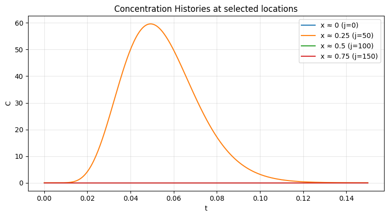
# Plots (helpers from earlier)
_ = plot_profiles(C, x, times=[0.0, 0.2, 0.4, 0.6], dt=dt, title="Upwind formulation advection")
_ = plot_histories(C, x, x_locs=[0.0, 0.25, 0.50, 0.75], dt=dt, by="coord")

../../_images/a91ba0b16636dec0898796f0c444cc6cc9bc1cf09cff32218efe5ffc269cefaf.png

../../_images/0546cf302e001ed52e7c8ed27703934861a276e86b99f4658444ee21580c9356.png

Centered formulation#

\[C_i^{n+1} = C_i^n + \frac{\Delta t}{2 \Delta x}(V_{i-1}*C_{i-1}^n - V_{i}*C_{i+1}^n)\]

This scheme will exhibit substantial numerical diffusion in part because it is a non-upwind formulation.

Below is a simple spreadsheet implementation of the explicit, centered in space scheme above.

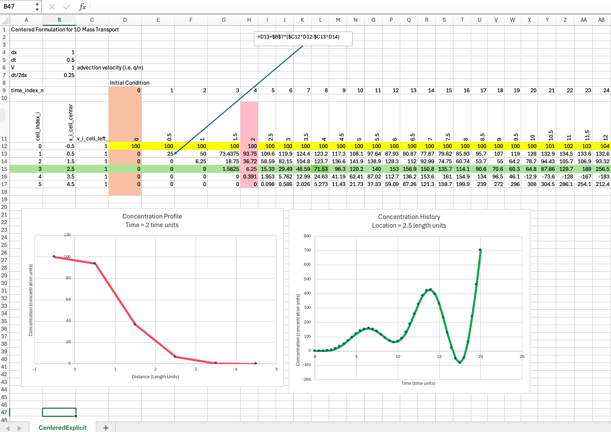
The spreadsheet above nicely exhibits numerical diffusion, apparent in the profile plot as well as oscillation in the time history. Professional tools address this phenomenon by a variety of approaches, upwinding and flux limiters being common reliable methods, a method of characteristics is another way to deal with the issue.

Below is a centered-difference (Forward Time Centered Space) version (of the python example) that demonstrates oscillations and instability (and “worse” numerical dispersion) compared to upwind formulations. It uses the conservative flux form with a centered interface flux:

$F_{i+\frac{1}{2}} =\frac{1}{2} V_{i+\frac{1}{2}} \cdot (C_i + C_{i+1})$

The update portion is same as above.

import numpy as np

def central_1d(
    C0: np.ndarray,
    v,                     # scalar, (nx,), (nt,), or (nt, nx) — same conventions as before
    dx: float,
    dt: float,
    nt: int,
    C_left=None,           # left Dirichlet BC: scalar or array length nt/nt+1; default = hold C0[0]
    C_right=None           # right Dirichlet BC: scalar or array length nt/nt+1; default = outflow (zero-gradient)
) -> np.ndarray:
    """
    Forward-Time / Centered-Space (FTCS) for 1D advection in conservative form:
        C^{n+1}_i = C^n_i + (dt/dx) * (F_{i-1/2} - F_{i+1/2})
    with centered interface flux:
        F_{i+1/2} = 0.5 * v_{i+1/2} * (C_i + C_{i+1})

    IMPORTANT: FTCS for pure advection is unconditionally unstable.
    Use for demonstration of oscillations/instability and dispersive artifacts.

    Parameters
    ----------
    C0 : (nx,) array
        Initial concentration at t=0.
    v : scalar | (nx,) | (nt,) | (nt,nx)
        Velocity evaluated at interfaces (i+1/2). Same broadcasting rules as in the upwind solver.
    dx, dt : float
        Grid spacing and time step.
    nt : int
        Number of steps.
    C_left, C_right : scalar | array | None
        Dirichlet BCs. If None:
          - left defaults to holding C[0] at its initial value (Dirichlet)
          - right defaults to zero-gradient outflow (C[-1] = C[-2] at each step)

    Returns
    -------
    C : (nt+1, nx) array
        Solution including initial state.
    """
    C0 = np.asarray(C0, dtype=float)
    nx = C0.size
    if nx < 2:
        raise ValueError("C0 must have length >= 2.")

    v_arr = _broadcast_velocity(v, nt, nx)

    # Boundary series
    left_series  = _expand_bc(C_left,  nt, default=C0[0])  # Dirichlet or hold
    right_series = _expand_bc(C_right, nt, default=None)   # None => outflow

    # Heads-up for students: FTCS is unstable (CFL won't save it)
    umax = np.nanmax(np.abs(v_arr))
    if umax > 0:
        print("⚠️ Note: FTCS (centered) for advection is unconditionally unstable.")
        print(f"   Courant max = {(umax*dt/dx):.3f} (shown for reference only).")

    C = np.zeros((nt+1, nx), dtype=float)
    C[0] = C0

    for n in range(nt):
        # Enforce BCs at current time level BEFORE computing fluxes
        C[n, 0] = left_series[n]
        if right_series is None:
            C[n, -1] = C[n, -2]       # zero-gradient outflow (ghost equal to interior)
        else:
            C[n, -1] = right_series[n]

        # Interface velocities for this step (i = 0..nx-2)
        v_n = v_arr[n, :]

        # Centered interface flux: F[i] = 0.5 * v[i] * (C[i] + C[i+1])
        F = 0.5 * v_n[:-1] * (C[n, :-1] + C[n, 1:])   # length nx-1

        # Update interior cells
        C[n+1, 1:-1] = C[n, 1:-1] + (dt/dx) * (F[:-1] - F[1:])

        # Next-time BCs
        C[n+1, 0] = left_series[n+1]
        if right_series is None:
            C[n+1, -1] = C[n+1, -2]
        else:
            C[n+1, -1] = right_series[n+1]

    return C


# ---- helpers (same as earlier; include here if not already defined) ----

def _broadcast_velocity(v, nt, nx):
    """
    Return velocity array of shape (nt, nx).
    Interprets v[n, i] at interfaces i=0..nx-2 (last column unused).
    """
    if np.isscalar(v):
        return np.full((nt, nx), float(v))
    v = np.asarray(v, dtype=float)
    if v.ndim == 1:
        if v.size == nx:
            return np.repeat(v[np.newaxis, :], nt, axis=0)
        if v.size == nt:
            return np.repeat(v[:, np.newaxis], nx, axis=1)
        raise ValueError("v length must be nx or nt if 1D.")
    if v.ndim == 2 and v.shape == (nt, nx):
        return v
    raise ValueError("v must be scalar, (nx,), (nt,), or (nt,nx).")

def _expand_bc(bc, nt, default=None):
    """
    Normalize BC to a series of length nt+1.
    - None: left -> hold default; right -> None (signals outflow)
    - scalar: constant series
    - array: length nt or nt+1 accepted
    """
    if bc is None:
        return None if default is None else np.full(nt+1, float(default))
    if np.isscalar(bc):
        return np.full(nt+1, float(bc))
    bc = np.asarray(bc, dtype=float).ravel()
    if bc.size == nt:
        return np.concatenate([bc, bc[-1:]])
    if bc.size == nt + 1:
        return bc
    raise ValueError("Boundary series must be scalar or length nt or nt+1.")

# Grid & initial rectangular pulse
nx = 201
x  = np.linspace(0.0, 1.0, nx)
dx = x[1] - x[0]

def rectangular_pulse_centered(x, x0, width, C0=1.0):
    half = 0.5*width
    return C0 * ((x >= x0-half) & (x <= x0+half)).astype(float)

C0 = rectangular_pulse_centered(x, x0=0.25, width=0.10, C0=1.0)

# Velocity & time
v  = 1.0
dt = 0.4 * dx / abs(v)   # (CFL shown for reference; FTCS still unstable)
nt = 200

# Solve with centered FTCS
C_cen = central_1d(C0, v, dx, dt, nt, C_left=0.0)

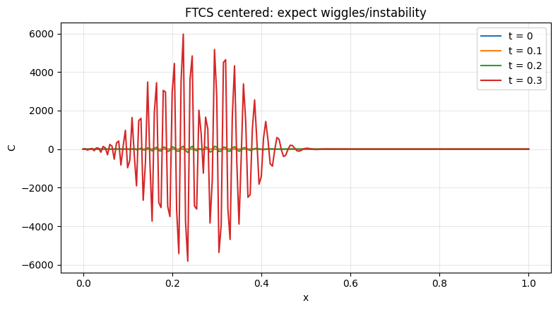
# Plot (using your earlier helpers)
_ = plot_profiles(C_cen, x, times=[0.0, 0.1, 0.2, 0.3], dt=dt, title="FTCS centered: expect wiggles/instability")
_ = plot_histories(C_cen, x, x_locs=[0.25, 0.5, 0.75], dt=dt, by="coord", title="Histories (FTCS centered)")

⚠️ Note: FTCS (centered) for advection is unconditionally unstable.
   Courant max = 0.400 (shown for reference only).

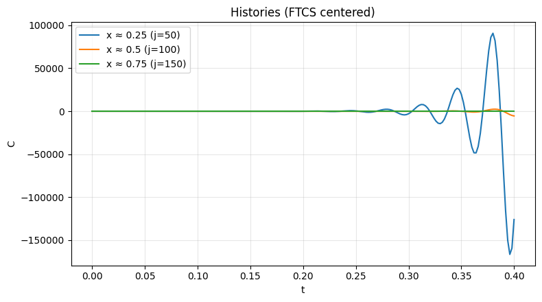
../../_images/25d4aeec60ad5e7ebcd224e1fff98ce0a59e37553a8fd8dfb5d8cb6ad18f3bb1.png

../../_images/9e1d8afe2c08795024c339e240244ca2045a167c71126982118add6088693807.png

Numerical Diffusion When solving advection-dominated partial differential equations (PDEs) using numerical methods, one common issue is numerical diffusion (also called numerical dissipation). This artifact of the numerical scheme can significantly affect the accuracy of the solution, particularly when sharp gradients or fronts are present, as in contaminant transport or shock waves.

Numerical diffusion is especially problematic in non-upwind formulations, such as those using central differencing for spatial derivatives. To understand why this happens, let’s review what numerical diffusion is and why it arises in these schemes. What is Numerical Diffusion?

Numerical diffusion refers to the artificial smoothing or blurring of a solution in a numerical model, which leads to a loss of sharpness in the advective transport of quantities like contaminants, pollutants, or heat. This effect is not physical but arises from the discretization of the advection equation.

The equation should transport $C(x,t)$ without changing its waveform (if no other processes, such as diffusion or dispersion, are acting). However, many numerical schemes, particularly non-upwind methods, introduce spurious diffusion into the solution.

Central Differencing and Numerical Diffusion

One popular method for approximating the spatial derivative is central differencing which is used in the scheme just preceding. While central differencing has second-order accuracy, meaning it can provide higher accuracy for smooth solutions, it is unstable when applied to advection-dominated problems without additional stabilization mechanisms. Specifically, central differencing often leads to oscillations and numerical diffusion in the solution when dealing with sharp fronts or discontinuities.

Why Numerical Diffusion Occurs

Numerical diffusion arises from the fact that non-upwind methods, like central differencing, do not adequately account for the direction of the flow in advection-dominated problems. In these cases, the finite-difference scheme inadvertently mimics a diffusive process. This can be understood as follows:

Information propagation: In hyperbolic PDEs like the advection equation, information propagates in a specific direction (determined by the sign of cc). Non-upwind methods like central differencing treat the spatial derivative symmetrically, which leads to a lack of proper alignment with the flow direction.
Smoothing effect: When central differencing is used in such cases, it smooths the solution because it averages information from both directions (upstream and downstream) of the grid point. This acts similarly to a diffusion process, where sharp gradients are smeared over time.

Impact of Numerical Diffusion

Numerical diffusion is particularly problematic for sharp fronts, such as contaminant plumes, where it can cause:

Excessive smoothing of the front: The sharp boundary of the plume becomes diffused over a larger area than physically expected.
Loss of mass conservation: In some cases, numerical diffusion can lead to non-conservative solutions, where the total amount of the transported quantity is not accurately preserved.

For example, if you are modeling the transport of a pollutant in groundwater using central differencing, the sharp concentration gradient between the polluted and unpolluted regions can be artificially blurred. This causes the plume to spread out more than it physically should.

Mitigating Numerical Diffusion

To reduce or eliminate numerical diffusion, upwinding schemes are commonly used. The upwind finite-difference method ensures that the spatial derivative is calculated using values from the upstream direction, thus preventing the unwanted smoothing that central differencing introduces. Although upwinding itself introduces some numerical dissipation, this dissipation is somewhat controlled and aligned with the flow direction, making it more suitable for advection-dominated problems.

Marker-in-Cell and Method of Characteristic models are hybrids that leverage a particle tracking approach to locate mean values, then dispersion about that mean value to honor the hyperbolic component while preserving the diffusion-like nature of the non-advective terms.

Summary: Advection Modeling—Particles vs. Grids (and Hybrids)#

Two viewpoints

Lagrangian (particle tracking): follow particles through a velocity field (from heads).
- Strengths: exact advection along pathlines; travel times/paths are natural outputs; easy to include decay along trajectories.
- Limits: no Eulerian concentration field unless you bin/Kernel-density the particles; mixing/dispersion must be modeled explicitly.
Eulerian (finite differences on a grid): evolve $C(x,t)$ on cells.

Strengths: full fields for mass balances, boundary/source terms, reactions, diffusion/dispersion.
Limits: subject to numerical diffusion/dispersion and stability constraints (CFL).

Two finite-difference advection schemes above:

Upwind (first-order)

Stable under $|v|\frac{\Delta t}{\Delta x} \le 1$
Introduces numerical diffusion (controlled and aligned with flow).
Good baseline for advection-dominated problems when you must avoid spurious wiggles.
Rule-of-thumb: effective artificial diffusion scales like $D_{num} \approx \frac{1}{2} |v| \Delta x$ (order of magnitude)

Forward time centered space (FTCS)

Unconditionally unstable for pure advection; exhibits oscillations/odd–even wiggles.
Useful as a counterexample to show why upwinding (or better schemes) are employed.

To suppress spurious oscillations in advection, practitioners commonly use upwinding. It does add dissipation, but in a controlled, flow-aligned way. To reduce that dissipation without re-introducing wiggles, move to higher-order upwind (e.g., Lax–Wendroff with limiters, MUSCL/TVD, flux limiters).

Hybrids that bridge the views

Marker-in-Cell / Particle-in-Cell and Method of Characteristics (MOC):

Carry advective motion with particles/characteristics, then deposit/average to the grid to handle diffusion/reaction.
Preserve sharp fronts better than low-order Eulerian schemes while still giving a grid-based $C(x,t)$.

When to use what (decision guide)

Only care about paths & travel times → Particle tracking (simpler, fast, minimal numerics).
Need concentrations, sources/sinks, reactions, diffusion → Eulerian grid (start with upwind; consider TVD/limited higher-order if fronts matter).
Advection-dominated with fronts + need $C(x,t)$ → Hybrids (MOC/MiC/PIC) or TVD schemes.

Practical reminders:

Always report the Courant number $CFL = |v|\frac{\Delta t}{\Delta x}$ and the cell Péclet number $Pe_{cell}=∣v∣Δx/D$ when diffusion is present.
Check mass conservation (Eulerian) or particle count (Lagrangian) to diagnose numerical artifacts.
Choose the method to match the question: pathlines vs. plume shape and concentrations.

Tip

If your goal is travel times and flow paths, particle methods are often the most direct and transparent—even if you give up the convenience of a full Eulerian concentration field.

Extension to 2 Spatial Dimensions#

Note

Extension of the upwind to 2D is shown below as a work-in-progress

Method: 2-D first-order upwind (Godunov/flux-splitting) solver for advection with velocities $(u,v)$ on a uniform $(x,y)$ grid, plus a contour plotting prototype function.
Defaults: Dirichlet on the left and bottom (held to initial boundary values if you don’t pass BCs) and advective outflow (zero-gradient) on the right and top.
Face velocities are computed by averaging adjacent cell-center values; if you already have $u,v$ on faces, you can pass them via (nt,ny,nx) and replace the averaging with your face arrays (shifted appropriately).
Outflow copies the last interior row/column along the outward normal each step (zero gradient).
For spatially varying or time-varying velocities, pass u and v as (ny,nx) or (nt,ny,nx) (or (nt,) for uniform-in-space time series).
Stability: the solver prints a warning if max(|u|*dt/dx + |v|*dt/dy) > 1.

import numpy as np
import matplotlib.pyplot as plt

# =========================
# 2-D UPWIND ADVECTION
# =========================
def upwind_2d(
    C0: np.ndarray,        # shape (ny, nx) at t=0
    u, v,                  # scalar | (ny,nx) | (nt,) | (nt,ny,nx)
    dx: float, dy: float,
    dt: float, nt: int,
    C_left=None,           # Dirichlet at x=0: scalar | (ny,) | (nt+1,ny) | (nt,ny)
    C_right=None,          # Dirichlet at x=Lx; None => outflow
    C_bottom=None,         # Dirichlet at y=0: scalar | (nx,) | (nt+1,nx) | (nt,nx)
    C_top=None             # Dirichlet at y=Ly; None => outflow
) -> np.ndarray:
    """
    First-order upwind (Godunov) scheme in 2-D, explicit time-stepping.

    Conservative form:
        C^{n+1}_{j,i} = C^n_{j,i}
            + (dt/dx) * (F_x[j, i-1] - F_x[j, i])
            + (dt/dy) * (F_y[j-1, i] - F_y[j, i])

    Face fluxes (flux-splitting):
        F_x[j, i] = max(u_face[j,i], 0)*C[j, i] + min(u_face[j,i], 0)*C[j, i+1]
        F_y[j, i] = max(v_face[j,i], 0)*C[j, i] + min(v_face[j,i], 0)*C[j+1, i]

    where i indexes x (columns), j indexes y (rows).
    u_face has shape (ny, nx-1) on x-interfaces; v_face has shape (ny-1, nx) on y-interfaces.

    Velocity inputs u, v:
      - scalar: constant everywhere
      - (ny,nx): spatially varying, constant in time
      - (nt,): time-varying, uniform in space
      - (nt,ny,nx): fully varying in space & time
    u, v are treated as **cell-centered**; face velocities are arithmetic averages.

    Boundary conditions:
      - Left/Bottom default: Dirichlet, held to initial boundary values
      - Right/Top default: outflow (zero-gradient)

    Returns
    -------
    C : array, shape (nt+1, ny, nx)
        Concentration field over time, including t=0.
    """
    C0 = np.asarray(C0, dtype=float)
    ny, nx = C0.shape
    if ny < 2 or nx < 2:
        raise ValueError("C0 must be at least 2x2.")

    u_arr = _broadcast_vel_2d(u, nt, ny, nx)
    v_arr = _broadcast_vel_2d(v, nt, ny, nx)

    # Expand boundary condition time series
    left_series   = _expand_edge_bc(C_left,   nt, ny, default=C0[:, 0])   # (nt+1, ny)
    right_series  = _expand_edge_bc(C_right,  nt, ny, default=None)       # None => outflow
    bottom_series = _expand_edge_bc(C_bottom, nt, nx, default=C0[0, :])   # (nt+1, nx)
    top_series    = _expand_edge_bc(C_top,    nt, nx, default=None)       # None => outflow

    # CFL check: conservative 2-D explicit condition  max(|u|*dt/dx + |v|*dt/dy) <= 1
    umax = np.nanmax(np.abs(u_arr))
    vmax = np.nanmax(np.abs(v_arr))
    if (umax > 0 or vmax > 0):
        cfl = (umax * dt / dx) + (vmax * dt / dy)
        if cfl > 1.0 + 1e-12:
            print(f"⚠️ CFL warning: max(|u|*dt/dx + |v|*dt/dy) = {cfl:.3f} > 1. "
                  "Reduce dt or refine grid.")

    # Allocate solution
    C = np.zeros((nt+1, ny, nx), dtype=float)
    C[0] = C0

    for n in range(nt):
        # -- Apply BCs at current time level BEFORE fluxes --
        # Left (Dirichlet) or hold; Right (outflow unless Dirichlet)
        if left_series is not None:
            C[n, :, 0] = left_series[n]
        if right_series is None:
            C[n, :, -1] = C[n, :, -2]   # outflow
        else:
            C[n, :, -1] = right_series[n]

        # Bottom (Dirichlet) or hold; Top (outflow unless Dirichlet)
        if bottom_series is not None:
            C[n, 0, :] = bottom_series[n]
        if top_series is None:
            C[n, -1, :] = C[n, -2, :]   # outflow
        else:
            C[n, -1, :] = top_series[n]

        # -- Face velocities (cell-centered -> face-centered by averaging) --
        u_n = u_arr[n]  # (ny, nx)
        v_n = v_arr[n]  # (ny, nx)
        u_face = 0.5 * (u_n[:, :-1] + u_n[:, 1:])  # (ny, nx-1), x-interfaces
        v_face = 0.5 * (v_n[:-1, :] + v_n[1:, :])  # (ny-1, nx), y-interfaces

        # -- Fluxes --
        Fx = np.maximum(u_face, 0.0) * C[n, :, :-1] + np.minimum(u_face, 0.0) * C[n, :, 1:]
        Fy = np.maximum(v_face, 0.0) * C[n, :-1, :] + np.minimum(v_face, 0.0) * C[n, 1:, :]

        # -- Update interior cells (vectorized) --
        C[n+1, 1:-1, 1:-1] = (
            C[n, 1:-1, 1:-1]
            + (dt/dx) * (Fx[1:-1, :-1] - Fx[1:-1, 1:])
            + (dt/dy) * (Fy[:-1, 1:-1] - Fy[1:, 1:-1])
        )

        # -- Next-time BCs --
        if left_series is not None:
            C[n+1, :, 0] = left_series[n+1]
        if right_series is None:
            C[n+1, :, -1] = C[n+1, :, -2]
        else:
            C[n+1, :, -1] = right_series[n+1]

        if bottom_series is not None:
            C[n+1, 0, :] = bottom_series[n+1]
        if top_series is None:
            C[n+1, -1, :] = C[n+1, -2, :]
        else:
            C[n+1, -1, :] = top_series[n+1]

    return C


# ---------- Helpers ----------

def _broadcast_vel_2d(v, nt, ny, nx):
    """
    Broadcast v to shape (nt, ny, nx).
    Accepts: scalar | (ny,nx) | (nt,) | (nt,ny,nx)
    """
    if np.isscalar(v):
        return np.full((nt, ny, nx), float(v))
    v = np.asarray(v, dtype=float)
    if v.ndim == 2 and v.shape == (ny, nx):
        return np.repeat(v[np.newaxis, :, :], nt, axis=0)
    if v.ndim == 1 and v.size == nt:
        return np.repeat(v[:, np.newaxis, np.newaxis], ny, axis=1).repeat(nx, axis=2)
    if v.ndim == 3 and v.shape == (nt, ny, nx):
        return v
    raise ValueError("Velocity must be scalar, (ny,nx), (nt,), or (nt,ny,nx).")


def _expand_edge_bc(bc, nt, nedge, default=None):
    """
    Expand an edge Dirichlet BC to (nt+1, nedge).
    - bc=None:
        * if default is None -> return None (signals outflow)
        * else -> return constant array set to default values
    - bc scalar -> constant in time/space
    - bc 1D (nedge,) -> constant in time, varies along edge
    - bc 2D (nt,) or (nt+1,) -> uniform along edge over time
    - bc 2D (nt+1, nedge) or (nt, nedge) -> full specification
    """
    if bc is None:
        if default is None:
            return None
        default = np.asarray(default, dtype=float).ravel()
        if default.size != nedge:
            # Allow scalar default
            if default.size == 1:
                default = np.full(nedge, float(default))
            else:
                raise ValueError("Default BC length mismatch.")
        return np.repeat(default[np.newaxis, :], nt+1, axis=0)

    if np.isscalar(bc):
        arr = np.full((nt+1, nedge), float(bc))
        return arr

    bc = np.asarray(bc, dtype=float)
    # (nedge,) -> replicate over time
    if bc.ndim == 1 and bc.size == nedge:
        return np.repeat(bc[np.newaxis, :], nt+1, axis=0)

    # (nt,) or (nt+1,) -> uniform along edge over time
    if bc.ndim == 1 and (bc.size == nt or bc.size == nt+1):
        series = bc if bc.size == nt+1 else np.concatenate([bc, bc[-1:]])
        return np.repeat(series[:, np.newaxis], nedge, axis=1)

    # (nt, nedge) or (nt+1, nedge)
    if bc.ndim == 2 and bc.shape in [(nt, nedge), (nt+1, nedge)]:
        return bc if bc.shape[0] == nt+1 else np.vstack([bc, bc[-1:, :]])

    raise ValueError("Unsupported BC shape; see docstring for allowed forms.")


# =========================
# PLOTTING (contour at time t)
# =========================
def plot_contour_at_time(C, x, y, t_req, dt, levels=20, filled=True, ax=None, title=None):
    """
    Contour (or filled contour) of C(x,y,t) at the requested physical time.
    C shape: (nt+1, ny, nx); x: (nx,), y: (ny,)
    """
    C = np.asarray(C)
    y = np.asarray(y); x = np.asarray(x)
    nt = C.shape[0]-1

    k = int(round(t_req / dt))
    k = max(0, min(nt, k))
    t_used = k * dt

    if ax is None:
        fig, ax = plt.subplots(figsize=(6.5, 5.0))

    X, Y = np.meshgrid(x, y)
    if filled:
        cs = ax.contourf(X, Y, C[k], levels=levels)
    else:
        cs = ax.contour(X, Y, C[k], levels=levels)
    cbar = plt.colorbar(cs, ax=ax)
    cbar.set_label("C")

    ax.set_xlabel("x"); ax.set_ylabel("y")
    ax.set_title(title or f"C(x,y,t) at t ≈ {t_used:.3g}")
    ax.set_aspect('equal', adjustable='box')
    ax.grid(True, alpha=0.2)
    plt.tight_layout()
    return ax, t_used, k

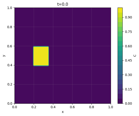
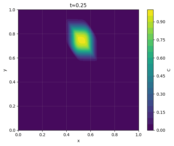
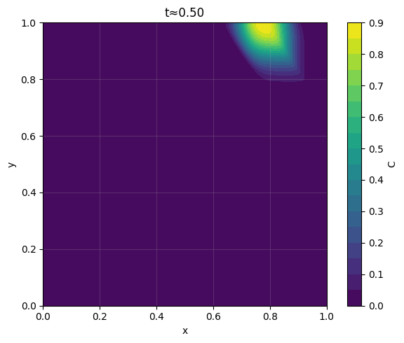
Minimal (testing) example: $(u,v)=(1,0.5)$, a rectangular patch as the initial condition, outflow on right/top.

# Grid
nx, ny = 121, 81
x = np.linspace(0.0, 1.0, nx)
y = np.linspace(0.0, 1.0, ny)
dx = x[1]-x[0]; dy = y[1]-y[0]

# Initial condition: 2-D rectangular patch
X, Y = np.meshgrid(x, y)
C0 = ((0.2 <= X) & (X <= 0.35) & (0.4 <= Y) & (Y <= 0.6)).astype(float)

# Velocities (cell-centered); constants here
u = 1.0
v = 0.5

# Time step from conservative 2-D CFL: |u|*dt/dx + |v|*dt/dy <= 1
CFL = 0.6
dt = CFL / (abs(u)/dx + abs(v)/dy)
nt = 250

# Left & bottom Dirichlet (hold at initial boundary); right & top: outflow
C = upwind_2d(C0, u, v, dx, dy, dt, nt,
              C_left=None, C_right=None, C_bottom=None, C_top=None)

# Plot at selected times
_ = plot_contour_at_time(C, x, y, t_req=0.0,   dt=dt, levels=20, filled=True, title="t=0.0")
_ = plot_contour_at_time(C, x, y, t_req=0.25,  dt=dt, levels=20, filled=True, title="t≈0.25")
_ = plot_contour_at_time(C, x, y, t_req=0.50,  dt=dt, levels=20, filled=True, title="t≈0.50")

../../_images/367fb6671eb72d4d3db46387680b7f58602db1c2da13b61ab5deda41355b8c96.png

../../_images/9f23e80141946debea69702d1da944d43a22bea515c275940e5d8f9831fc1f0a.png

../../_images/eefb5717a6525314ae0221ee255f34197c7c486280b724af5d779e1d62c8178d.png

Exercise(s)#

ce5364-es4-2025-3.pdf

# autobuild exercise
import subprocess

try:
    subprocess.run(["pdflatex", "ce5364-es4-2025-3.tex"], 
                   stdout=subprocess.DEVNULL, stderr=subprocess.DEVNULL, check=True)
except subprocess.CalledProcessError:
    print("Build failed. Check your LaTeX source file.")

Section End#

ce5364-es4-2025-3-ExampleReport.pdf PLACEHOLDER

8. Modeling Advection

Contents

8. Modeling Advection#

Readings#

Videos#

Methods#

Particle Tracking:#

Upwind Finite Difference:#

Modeling Advection by Particle Tracking (Lagrangian Approach)#

Multi-Linear Interpolation#

Spreadsheet (Excel) Approach#

Spreadsheet Examples#

Particle Tracking in Python#

Step 1. Need to Digitize the Head Map#

Step 2 Check the Digitization Results#

Extensions#

Modeling Advection by Finite-Difference (Eulerian Approach)#

Finite-Difference Method#

Upwinding in Hyperbolic-Dominant PDEs#

Why Upwinding is Important#

Upwind formulation#

Centered formulation#

Summary: Advection Modeling—Particles vs. Grids (and Hybrids)#

Extension to 2 Spatial Dimensions#

Exercise(s)#

Section End#