9. Analytical Solutions (1D)#
Partial Differential Equations (PDEs) are powerful mathematical tools used to describe and understand a wide range of physical phenomena, from heat diffusion to fluid flow. When dealing with PDEs, two primary approaches are commonly employed: analytical solutions and numerical models.
Course Website
%%html
<style> table {margin-left: 0 !important;} </style>
Readings#
Bear, J. (1972) Dynamics of Fluids in Porous Media McGraw Hill (pp. 628-629)
SSANTS2.xlsm (Excel Macro Sheet(s)) Contains several different models (and varying boundary conditions). Originally written in Excel94 Macro language, likely no longer runs in modern Excel (but may run in LibreOffice)
Videos#
Analytical Models#
Analytical solutions to PDEs involve finding exact mathematical expressions that describe the behavior of a system without resorting to approximation or numerical computation. These solutions are derived through mathematical techniques such as separation of variables, Fourier analysis, and Laplace transforms. The advantages of analytical solutions include:
Precision: Analytical solutions provide precise, closed-form expressions that yield exact solutions for specific initial and boundary conditions. This accuracy is particularly valuable in situations where precision is crucial, such as in fundamental scientific research or engineering design.
Insight: Analytical solutions offer deep insight into the underlying physics of the problem. They reveal how various parameters and variables influence the system’s behavior, facilitating a fundamental understanding of the problem at hand.
Computational Efficiency: Analytical solutions are typically computationally efficient, requiring significantly less computational power compared to numerical methods, which can be advantageous when working with complex or time-sensitive problems.
Numerical Models:#
Numerical models, on the other hand, involve discretizing the domain of the PDE into a grid or mesh and approximating the solution at discrete points. Numerical methods, such as finite difference, finite element, and finite volume methods, are used to solve the resulting system of algebraic equations. The key characteristics of numerical models include:
Approximation: Numerical models inherently involve approximation, as they operate with discretized values. The accuracy of the solution depends on the grid size and the chosen numerical method. Smaller grid sizes yield more accurate results but require more computational resources.
Versatility: Numerical models are versatile and can handle complex geometries and boundary conditions. They are particularly well-suited for solving PDEs that lack analytical solutions or when analytical solutions are impractical due to complexity.
Computational Resources: Numerical models can be computationally intensive, especially for high-resolution simulations or large-scale problems. High-performance computing resources may be necessary for timely solutions.
Comparison:#
The choice between analytical solutions and numerical models depends on the nature of the problem and the specific objectives of the analysis:
Analytical solutions are preferred when exact, closed-form expressions are achievable, offering precise insights into the system’s behavior. They are particularly useful for fundamental research and for understanding the underlying physics.
Numerical models excel when dealing with complex geometries or when no analytical solutions are available. They offer flexibility and can handle a wide range of practical problems, making them indispensable in engineering, environmental modeling, and simulating real-world scenarios.
Spatial Dimensionality#
Spatial dimensionality in modeling refers to the number of spatial dimensions or coordinates used to describe the physical or geometric aspects of a system or problem. In various scientific and engineering contexts, models are often used to represent and understand how a system behaves or evolves in space. Spatial dimensionality plays a crucial role in defining the complexity and realism of these models.
Here’s a breakdown of what spatial dimensionality means in modeling:
One-Dimensional (1D) Models: In one-dimensional models, the system or problem is simplified to a single spatial dimension. For example, a heat conduction model in a rod with heat varying only along its length can be represented as a 1D model. These models are suitable for problems with significant simplification in spatial variation.
Two-Dimensional (2D) Models: In two-dimensional models, the system is represented in two spatial dimensions, typically on a flat plane. This is common in scenarios where variations occur both horizontally and vertically. Examples include flow in a thin aquifer or heat diffusion on a flat surface.
Three-Dimensional (3D) Models: Three-dimensional models account for variations in three spatial dimensions, forming a 3D space. These models are used for systems with complex spatial variations in all three directions. Examples include simulating groundwater flow in a 3D aquifer or airflow in a 3D room.
Higher-Dimensional Models: In some cases, particularly in theoretical physics and mathematics, models may involve more than three spatial dimensions. Such models are rare in practical applications but can be used to explore abstract or theoretical concepts.
The choice of spatial dimensionality in modeling depends on the nature of the problem being studied and the level of detail required to capture its essential characteristics. Simplifying a problem to fewer dimensions can make it more tractable and computationally efficient but may lead to a loss of accuracy if important spatial variations are neglected. On the other hand, using a higher spatial dimensionality can provide a more realistic representation of a complex system but may come at the cost of increased computational complexity.
Concentration Profiles#
In transport modeling, a “concentration profile” refers to the spatial distribution of the concentration of a substance (such as a solute or pollutant) within a medium at a specific point in time. It represents how the concentration of the substance varies across different locations or spatial coordinates within the medium.
The concentration profile is a fundamental concept in the study of transport phenomena, particularly in fields like hydrogeology, environmental science, and chemical engineering. It provides crucial information about how substances disperse, spread, or migrate through various media, such as air, water, soil, or porous materials. Understanding concentration profiles is essential for assessing the movement and behavior of substances in the environment and predicting their impact on ecosystems, human health, or industrial processes.
Key characteristics of a concentration profile include:
Spatial Variation: A concentration profile shows how the concentration of the substance changes as you move from one location to another within the medium. It typically represents this variation along one or more spatial dimensions (e.g., depth, distance, height, or time).
Peak Concentration: The concentration profile often indicates where the highest concentration of the substance occurs within the medium, which is known as the “peak concentration” or “maximum concentration.”
Concentration Gradients: Concentration profiles also reveal the gradients or slopes in concentration, indicating the rate at which the concentration changes over distance or time. Steeper gradients imply faster changes.
Boundary Conditions: The shape and characteristics of the concentration profile are influenced by various factors, including initial conditions, boundary conditions (e.g., sources or sinks), and the transport processes at play (e.g., advection, dispersion, diffusion).
Temporal Evolution: Concentration profiles can change over time as substances are transported, mixed, or degraded within the medium. Dynamic modeling often involves tracking how these profiles evolve.
Concentration profiles are commonly visualized using graphs or plots, with concentration (C) on the y-axis and spatial coordinates (e.g., distance or depth) on the x-axis. The resulting graph provides a visual representation of how the substance’s concentration varies spatially, helping researchers and modelers gain insights into the behavior and fate of the substance in the system.
Concentration Histories#
In transport modeling, “concentration history” refers to the temporal evolution or record of the concentration of a substance (such as a solute or pollutant) at a specific location or point within a medium over a period of time. It provides information about how the concentration of the substance changes at that particular location as time progresses.
The concentration history is a critical aspect of transport modeling and is used to track and analyze how the concentration of a substance responds to various transport and fate processes, including advection, dispersion, diffusion, chemical reactions, and source/sink terms. It is particularly relevant in fields such as environmental science, hydrogeology, chemical engineering, and pollution assessment. Understanding concentration histories is essential for predicting the behavior of contaminants, the spread of pollutants, and the effectiveness of remediation or mitigation measures.
Key characteristics and components of a concentration history include:
Temporal Variation: The concentration history shows how the concentration of the substance changes over time at a specific location. This temporal variation can reveal important trends, fluctuations, or trends in concentration levels.
Initial Conditions: The concentration history often begins with an initial concentration value at the starting time (t=0). This initial condition represents the state of the substance at the beginning of the simulation or observation period.
Transport Processes: Changes in concentration over time are influenced by various transport processes, including advection (bulk movement of fluid), dispersion (mechanical mixing), diffusion (molecular movement), chemical reactions, and any sources or sinks of the substance.
Boundary Conditions: Concentration histories are also affected by boundary conditions, which may include inflows, outflows, or other interactions at the system’s boundaries.
Equations and Models: Concentration histories are typically generated using mathematical models that describe the relevant transport and fate processes. These models are often based on partial differential equations or discrete numerical methods.
Concentration histories can be visualized using plots or graphs, with time (t) on the x-axis and concentration (C) on the y-axis. This graphical representation allows modelers and researchers to observe concentration trends and patterns. Concentration histories are essential for various applications, such as assessing the impact of contaminants on groundwater quality, tracking the dispersion of pollutants in surface water bodies, monitoring the progress of chemical reactions in industrial processes, and evaluating the performance of remediation strategies.
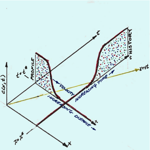
The image above is an illustration of the \(x-t\) plane, with the vertical axis the \(C(x,t)\) axis. At the source, the concentration is some fixed value. From the origin, moving upward and to the right is the time axis. From the origin, moving downward and to the right is the space (distance) axis. A yellow line in the \(x-t\) plane is \(x=vt\) (sometimes called the trajectory). Along the time axis, is a point in time indicated by \(t^*\). From this point moving downward and to the right is a plot (increasing distance) which is a concentration profile plot. Along the space axis, is a point in space indicated by \(x^*\). From this point moving upward and to the right is a plot (increasing time) which is a concentration history plot.
Selected One Dimensional Solutions#
What follows are some selected solutions. Most were built by convolution of an elementary impulse solution (which we start with) with the convolution integral built based on various boundary conditions - its probably an obsolete skill given today’s reliance on numerical models and effective symbolic manipulation programs.
Note
Why start with the impulse solution?
The delta (impulse) solution is the PDE’s “unit test.” Once we understand it, we can generate many other solutions by convolution with initial/boundary data.
Learning goals
See how the impulse solution enforces mass conservation, causality, and the PDE itself.
Practice verifying a proposed solution by checking the PDE, ICs/BCs, and limiting cases.
Use a computer algebra system (e.g., Mathematica, SymPy) or an LLM assistant to handle the mechanics (differentiation, integrals), while you supply modeling judgment.
On tools vs. hand work
Doing the full 1-D impulse derivation by hand can take hours and is valuable once. Modern tools confirm the same steps in seconds—freeing you to focus on formulation, assumptions, and interpretation rather than algebra.
Takeaway
Master the structure—impulse → convolution → apply IC/BC → verify. Then let software accelerate the calculations without skipping the checks.
1D Impulse (Instantaneous Source) Solution#
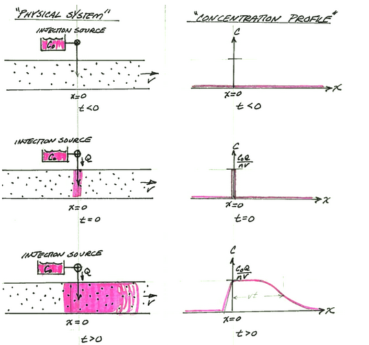
The figure below depicts the physical system as the three panels on the left, and the analytical model system at times larger than or equal to zero times.
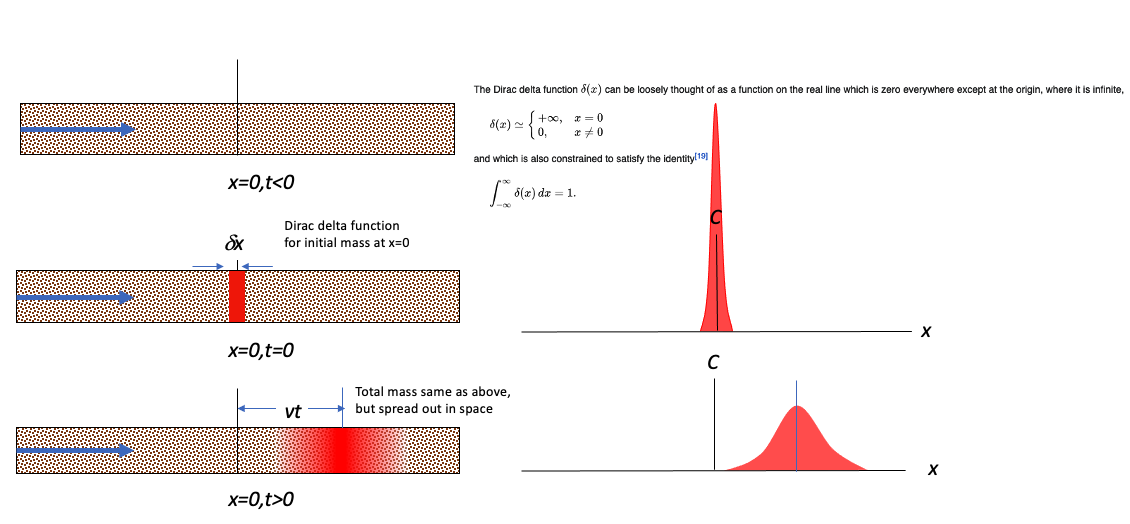
Upper Left Panel is a depiction of the physical system at time less than zero. The concentration is zero everywhere, and the cooresponding profile is not plotted
Middle Left Panel is a depiction of the physical system and the concentration profile along the x-axis at time equal zero (like the Big Bang!). At x = 0, the concentration is suddenly raised to a value of \(C_0 \cdot \delta x = \frac{M}{A}\) at the origin, x=0. This condition represents a Dirac delta function input and is a suitable approximation of a sudden release in a source zone that has a constant concentration. The concentration away from the origin is still zero. The right middle panel is a profile plot of concentration (the Delta function is unplottable, so the cartoon must suffice).
Bottom Left Panel is a depiction of the physical system and the concentration profile along the x-axis at some time greater than zero. The source mass center has moved to the right of the origin a distance determined by the species velocity and dispersed along the translational front proportional to the dispersivity in the system.
The analytical solution for this situation is given in Bear, J. (1972) Dynamics of Fluids in Porous Media McGraw Hill (pp. 628-629)
It is also presented in the textbook as equation 6.18
where
\(M\) is mass injected per unit cross-sectional area,
\(D_x = \alpha_L*v+D_d\) is the hydrodynamic dispersion (plus any molecular diffusion),
\(v = \frac{q}{n}\) is the pore velocity
The solution is applicable for porous media flow, where the velocity is the pore velocity (seepage velocity divided by the porosity).
Note
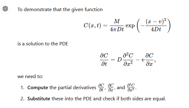
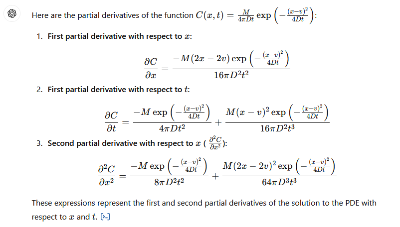
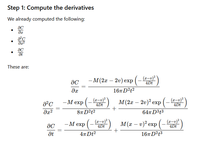
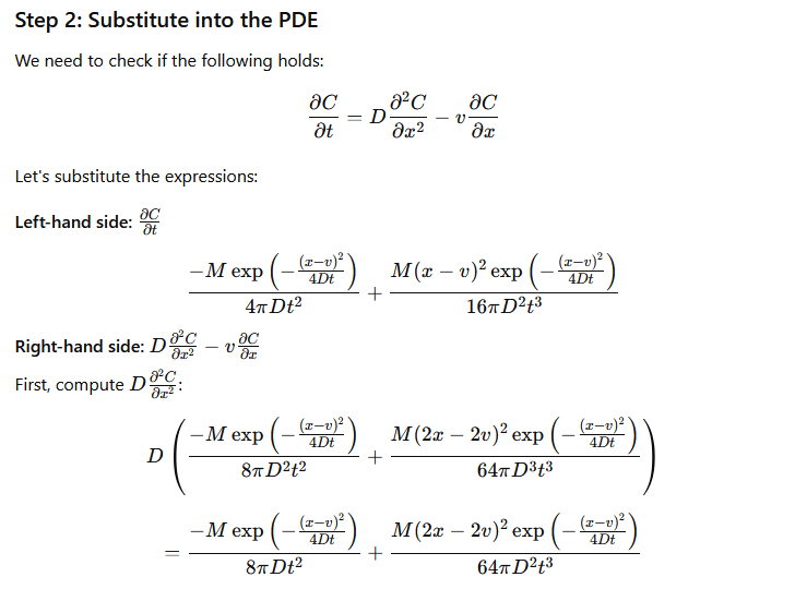
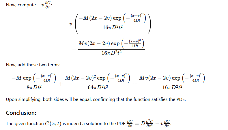
We should check that it is a solution to
by differentiating the solution once by \(x\) then that result again by \(x\), then once by \(t\), and putting these results back into the ADE to verify that the result indeed fits the PDE.
The process is illustrated below (I have not checked the math, but the process is straightforward) using GPT-4.0; Mathematica is probably a better tool for this exercise, but its API doen not interpret natural language input very well.
Verify Solution#
OpenAI. (2024). ChatGPT (GPT-4).
The images below are a transaction transcript (the prompt was)
Can you demonstrate that C(x,t)=M/(4*pi*D*t) * exp(-(x-v)**2 /(4*D*t) where x,t are variables, M,pi,D,v are known constants is a solution to the PDE dC/dt = D d^2C/dx^2 - v dc/dx?
Retrieved [12 Sep 2024], from https://chat.openai.com
Building a Modeling Tool#
This particular model is all over the internet as an on-line calculator, but sometimes we have need to build our own version. In Jupyter Notebooks running a python kernel we need to script the equation above and structure the equation into a useable function.
Forward define the functions#
This step is important, the functions must be defined before they are called – in an interpreter, this is usually done at the top of the script. Other scripting languages store the scripts at the end (JavaScript usually keeps scripts at end of the file – it internally promotes then to the top before it runs its JIT bytecode compiler).
In a compiled language, this step is not as necessary (predefinition is, location not so much).
These prototype functions are usually written so that they are organic with respect to their variables, so there is no leakage – in these two functions, the input list is just names, and the output is just a value that must be assigned in the calling script.
def impulse1D(distance,time,mass,dispersion,velocity):
    import math
    term1 = math.sqrt(4.0*math.pi*dispersion*time)
    term2 = math.exp(-((distance-velocity*time)**2)/(4.0*dispersion*time))
    impulse1D = (mass/term1)*term2
    return(impulse1D)
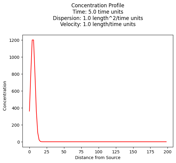
Concentration Profile#
Making a profile plot is fairly straightforward, a script to do so is listed below.
Consider a case where \(10,000~ppm\) of a conservative constituient is suddenly released into a volume of \(1~m^3\) of groundwater moving at a seepage (pore) velocity of \(1~\frac{m}{day}\) in a flow system with a dispersion coefficient of \(1~\frac{m^2}{day}\).
Produce a concentration profile for the system at 75 days.
thick       = 1.0
width       = 100.0
length      = 0.01 # small but non-zero
volume      = thick*width*length
porosity    = 1.0
c0          = 10000.0 # kg/m^3
mass        = (c0*volume)/(porosity)
#print(mass)
dispersion  = 1.0 #m^2/day
velocity    = 1.0 #m/day
deltax      = 2.0 #meters
howmany     = 100 #how many points to compute
x = [] #meters
for i in range(howmany):
    x.append(float(i)*deltax)

time        = 5.00 # days
acc = []
c = [0 for i in range(howmany)] #concentration
for i in range(howmany):
    c[i]=impulse1D(x[i],time,mass,dispersion,velocity)
    acc.append(c[i]*deltax)
print(sum(acc))
#
# Import graphics routines for picture making
#
from matplotlib import pyplot as plt
#
# Build and Render the Plot
#
plt.plot(x,c, color='red', linestyle = 'solid')  # make the plot object
plt.title(" Concentration Profile \n Time: " + repr(time) + " time units \n" + " Dispersion: " + repr(dispersion) + " length^2/time units \n" + " Velocity: " + repr(velocity) + " length/time units \n") # caption the plot object
plt.xlabel(" Distance from Source ") # label x-axis
plt.ylabel(" Concentration        ") # label y-axis
#plt.savefig("ogatabanksplot.png") # optional generates just a plot for embedding into a report
plt.show() # plot to stdio -- has to be last call as it kills prior objects
plt.close('all') # needed when plt.show call not invoked, optional here
#sys.exit() # used to elegant exit for CGI-BIN use
#print("Advective Front Position : ",round(time*velocity,2)," length units")
#print("Total Mass : ",round(mass,3)," kg")
9731.787793845493
Spreadsheet Model#
A spreadsheet model is located at http://54.243.252.9/ce-5364-webroot/6-Spreadsheets/ImpulseSolutionProfile.xlsx
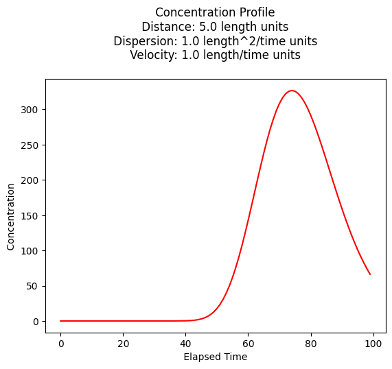
Concentration History#
Its also quite reasonable to build a history (concentration versus time at some location) - the script is practically the same, except time is the variable instead of space.
thick       = 1.0
width       = 100.0
length      = 0.01 # small but non-zero
volume      = thick*width*length
porosity    = 1.0
c0          = 10000.0 # kg/m^3
mass        = (c0*volume)/(porosity)
dispersion  = 1.0 #m^2/day
velocity    = 1.0 #m/day
deltat      = 1.0 #days
howmany     = 100 #how many points to compute
t = [] #meters
for i in range(howmany):
    t.append((float(i)+0.00001)*deltat)

space        = 75.0 # meters

c = [0 for i in range(howmany)] #concentration
for i in range(howmany):
    c[i]=impulse1D(space,t[i],mass,dispersion,velocity)
#
# Import graphics routines for picture making
#
from matplotlib import pyplot as plt
#
# Build and Render the Plot
#
plt.plot(t,c, color='red', linestyle = 'solid')  # make the plot object
plt.title(" Concentration Profile \n Distance: " + repr(time) + " length units \n" + " Dispersion: " + repr(dispersion) + " length^2/time units \n" + " Velocity: " + repr(velocity) + " length/time units \n") # caption the plot object
plt.xlabel(" Elapsed Time ") # label x-axis
plt.ylabel(" Concentration        ") # label y-axis
#plt.savefig("ogatabanksplot.png") # optional generates just a plot for embedding into a report
plt.show() # plot to stdio -- has to be last call as it kills prior objects
plt.close('all') # needed when plt.show call not invoked, optional here
#sys.exit() # used to elegant exit for CGI-BIN use
#print("Advective Front Position : ",round(time*velocity,2)," length units")
#print("Total Mass : ",round(mass,3)," kg")
Spreadsheet Model#
A spreadsheet model is located at http://54.243.252.9/ce-5364-webroot/6-Spreadsheets/ImpulseSolutionHistory.xlsx
1D Ogata-Banks Solution#
The figure below depicts the physical system, and the analytical model system at three different times.
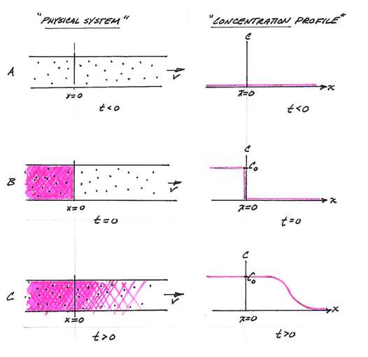
Panel A is a depiction of the physical system and the concentration profile along the x-axis at time less than zero. The concentration is zero everywhere.
Panel B is a depection of the physical system and the concentration profile along the x-axis at time equal zero (like the Big Bang!). At x < 0, the concentration is suddenly raised to a value of \(C_0\) everywhere to the left of the origin, x=0. This condition represents a step function input and is a suitable approximation of some upstream source zone that has a constant concentration. The concentration to the right of the origin (x > 0) is still zero.
Panel C is a depiction of the physical system and the concentration profile aling the x-axis at some time greater than zero. The source mass has moved to the right of the origin a distance determined by the species velocity and dispersed along the translational front proportional to the dispersivity in the system.
The analytical solution (Ogata and Banks, 1961) for this situation is:
where
\(C_0\) is the source concentration,
\(D_x = \alpha_L*v+D_d\) is the hydrodynamic dispersion (plus any molecular diffusion),
\(v = \frac{q}{n}\) is the pore velocity
It is also presented in the textbook as equation 6.17
The solution is applicable for porous media flow, where the velocity is the pore velocity (seepage velocity divided by the porosity).
Building a Model#
This particular model is also all over the internet as an on-line calculator, but sometimes we have need to build our own version. In Jupyter Notebooks running a python kernel we need to script the equation above and structure the equation into a useable function.
Forward define the functions#
This step is important, the functions must be defined before they are called – in an interpreter, this is usually done at the top of the script. Other scripting languages store the scripts at the end (JavaScript usually keeps scripts at end of the file – it internally promotes then to the top before it runs its JIT bytecode compiler).
In a compiled language, this step is not as necessary (predefinition is, location not so much).
These prototype functions are usually written so that they are organic with respect to their variables, so there is no leakage – in these two functions, the input list is just names, and the output is just a value that must be assigned in the calling script.
#
# prototype ogatabanks function
#
def ogatabanks(c_source,space,time,dispersion,velocity):
    from math import sqrt,erf,erfc,exp  # get special math functions
    term1 = erfc(((space-velocity*time))/(2.0*sqrt(dispersion*time)))
    term2 = exp(velocity*space/dispersion)
    term3 = erfc(((space+velocity*time))/(2.0*sqrt(dispersion*time)))
    #print(term3)
    ogatabanks = c_source*0.5*(term1+term2*term3)
    return(ogatabanks)
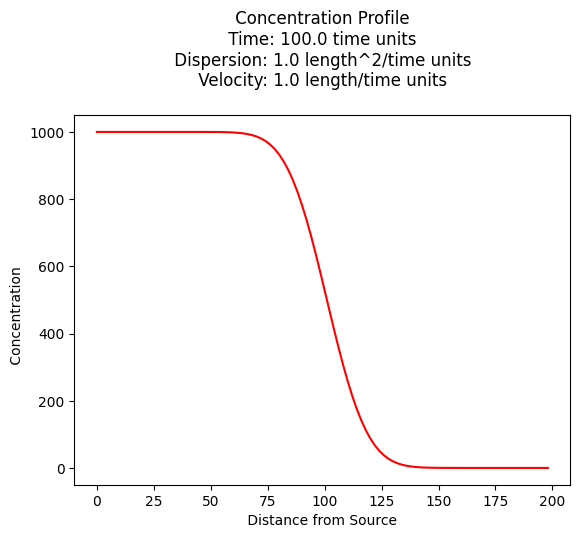
Concentration Profile#
The example below uses the function named ogatabanks to compute values for \(x \ge 0\) and \(t \gt 0\), and plot the resulting concentration profile.
#
# example inputs
#
c_source = 1000.0 # source concentration
space = 200.      # how far in X-direction to extend the plot
time  = 100.       # time since release
dispersion = 1.0  # dispersion coefficient
velocity = 1.0    # pore velocity
#
# forward define and initialize vectors for a profile plot
#
how_many_points = 100
deltax = space/how_many_points
x = [i*deltax for i in range(how_many_points)] # constructor notation
c = [0.0 for i in range(how_many_points)]      # constructor notation
#
# build the profile predictions
#
for i in range(0,how_many_points,1):
    c[i] = ogatabanks(c_source,x[i],time,dispersion,velocity)
#
# Import graphics routines for picture making
#
from matplotlib import pyplot as plt
#
# Build and Render the Plot
#
plt.plot(x,c, color='red', linestyle = 'solid')  # make the plot object
plt.title(" Concentration Profile \n Time: " + repr(time) + " time units \n" + " Dispersion: " + repr(dispersion) + " length^2/time units \n" + " Velocity: " + repr(velocity) + " length/time units \n") # caption the plot object
plt.xlabel(" Distance from Source ") # label x-axis
plt.ylabel(" Concentration        ") # label y-axis
#plt.savefig("ogatabanksplot.png") # optional generates just a plot for embedding into a report
plt.show() # plot to stdio -- has to be last call as it kills prior objects
plt.close('all') # needed when plt.show call not invoked, optional here
#sys.exit() # used to elegant exit for CGI-BIN use
Spreadsheet Model#
A spreadsheet model is located at http://54.243.252.9/ce-5364-webroot/6-Spreadsheets/OgataBanksProfile.xlsx
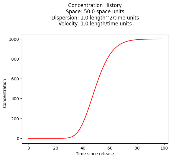
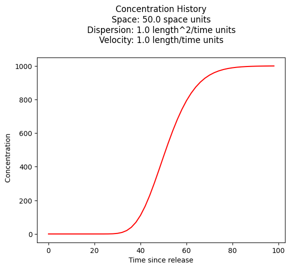
Concentration History#
Its also quite reasonable to build a history (concentration versus time at some location) - the script is practically the same, except time is the variable instead of space.
#
# example inputs
#
c_source = 1000.0 # source concentration
space = 50.      # where in X-direction are we
time  = 100.      # how far in T-direction to extend the plot
dispersion = 1.0  # dispersion coefficient
velocity = 1.0    # pore velocity
#
# forward define and initialize vectors for a profile plot
#
how_many_points = 50
deltat = time/how_many_points
t = [i*deltat for i in range(how_many_points)] # constructor notation
c = [0.0 for i in range(how_many_points)]      # constructor notation

t[0]=1e-5 #cannot have zero time, so use really small value first position in list
#
# build the profile predictions
#
for i in range(0,how_many_points,1):
    c[i] = ogatabanks(c_source,space,t[i],dispersion,velocity)
#
# Import graphics routines for picture making
#
from matplotlib import pyplot as plt
#
# Build and Render the Plot
#
plt.plot(t,c, color='red', linestyle = 'solid')  # make the plot object
plt.title(" Concentration History \n Space: " + repr(space) + " space units \n" + " Dispersion: " + repr(dispersion) + " length^2/time units \n" + " Velocity: " + repr(velocity) + " length/time units \n") # caption the plot object
plt.xlabel(" Time since release ") # label x-axis
plt.ylabel(" Concentration        ") # label y-axis
#plt.savefig("ogatabanksplot.png") # optional generates just a plot for embedding into a report
plt.show() # plot to stdio -- has to be last call as it kills prior objects
plt.close('all') # needed when plt.show call not invoked, optional here
#sys.exit() # used to elegant exit for CGI-BIN use
Example 6.1 (Using Near-Field Solution above)#
From pp. 174-175:
\(K=2.15~\frac{m}{day}\)
\(n=0.1\)
\(\frac{dh}{dx}=0.04\)
\(C_0=1000~ppm\)
\(\alpha_L = 7.5~m\)
Plot a concentration profile at 728 days.
Solution#
A little preparatory arithmetic is used:
\(v = \frac{1}{n} \cdot K \cdot \frac{dh}{dx} = \frac{1}{0.1} \cdot 2.15 \cdot 0.04 = 0.86~\frac{m}{day}\)
\(D~\approx~\alpha_L \cdot v = 7.5 \cdot 0.86 = 6.45~\frac{m^2}{day}\)
Now just use our program
#
# example inputs
#
c_source = 1000.0 # source concentration
space = 1500.      # how far in X-direction to extend the plot
time  = 728.       # time since release
dispersion = 6.45  # dispersion coefficient
velocity = 0.86   # pore velocity
#
# forward define and initialize vectors for a profile plot
#
how_many_points = 100
deltax = space/how_many_points
x = [i*deltax for i in range(how_many_points)] # constructor notation
c = [0.0 for i in range(how_many_points)]      # constructor notation
#
# build the profile predictions
#
for i in range(0,how_many_points,1):
    c[i] = ogatabanks(c_source,x[i],time,dispersion,velocity)
#
# Import graphics routines for picture making
#
from matplotlib import pyplot as plt
#
# Build and Render the Plot
#
plt.plot(x,c, color='red', linestyle = 'solid')  # make the plot object
plt.title(" Concentration Profile \n Time: " + repr(time) + " time units \n" + " Dispersion: " + repr(dispersion) + " length^2/time units \n" + " Velocity: " + repr(velocity) + " length/time units \n") # caption the plot object
plt.xlabel(" Distance from Source ") # label x-axis
plt.ylabel(" Concentration        ") # label y-axis
#plt.savefig("ogatabanksplot.png") # optional generates just a plot for embedding into a report
plt.show() # plot to stdio -- has to be last call as it kills prior objects
plt.close('all') # needed when plt.show call not invoked, optional here
#sys.exit() # used to elegant exit for CGI-BIN use

print("Concentration at x = 750, t = 728 :",round(ogatabanks(c_source,750.0,728.0,dispersion,velocity),3)," mg/L")
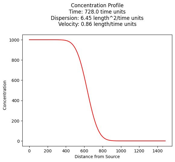
Concentration at x = 750, t = 728 : 112.838 mg/L
Compare the result to the textbook, which uses the far-field solution for a value of \(100~mg/L\) (how would you modify for the far-field solution?)
Spreadsheet Model#
A spreadsheet model is located at http://54.243.252.9/ce-5364-webroot/6-Spreadsheets/OgataBanksHistory.xlsx
1D Sauty Solution#
A slightly different condition occurs when the constituient is added at x=0 at a constant rate. The figure below depicts the physical system, and the analytical model system at three different times.
Panel A is a depiction of the physical system and the concentration profile along the x-axis at time less than zero. The concentration is zero everywhere. An injection supply is depicted by the small reservoir and the injection path into the aquifer (or stream). The valve is closed in this panel.
Panel B is a depection of the physical system and the concentration profile along the x-axis at time equal zero (like the Big Bang!). At t=0, mass is added into the aquifer (stream) at a rate CoQ at the origin (x=0). This mass flow rate at the injection site is maintained from t=0 onward.
Panel C is a depiction of the physical system and the concentration profile along the x-axis at some time greater than zero. The concentration front translates to the right of the origin a distance determined by the species velocity and dispersed along the front proportional to the dispersivity in the system. Some mass disperses upstream from the injection site.
The analytical solution (Sauty, 1980 ) for this situation is:
where
\(C_0\) is the source concentration,
\(D_x = \alpha_L*v+D_d\) is the hydrodynamic dispersion (plus any molecular diffusion),
\(v = \frac{q}{n}\) is the pore velocity
\(Q\) is the volumetric injection rate
\(n\) is the aquifer porosity
The solution is applicable for porous media flow, where the velocity is the pore velocity (seepage velocity divided by the porosity).
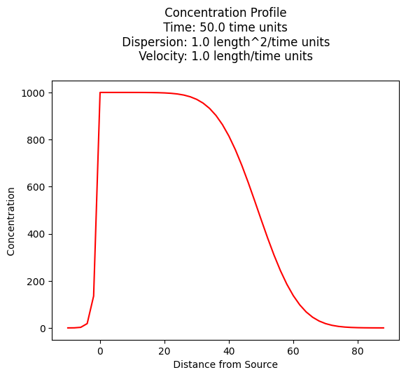
Concentration Profile#
The example below uses a function named sauty to compute values for \(x \ge 0\) and \(t \gt 0\), and plot the resulting concentration profile.
from math import sqrt,erf,erfc,exp  # get special math functions
#
# prototype sauty function
#
def sauty(c_source,injection,porosity,space,time,dispersion,velocity):
    term0 = (c_source*injection)/(2.0*porosity*velocity)
    term1 = exp( 0.5*velocity*space/dispersion)
    term3 = exp(-0.5*velocity*abs(space)/dispersion)
    term4 = erfc(((abs(space)-velocity*time))/(2.0*sqrt(dispersion*time)))
    term5 = exp( 0.5*velocity*abs(space)/dispersion)
    term6 = erfc(((abs(space)+velocity*time))/(2.0*sqrt(dispersion*time)))
    sauty = term0*term1*(term3*term4-term5*term6)
    return(sauty)
#
# example inputs
#
c_source = 1000.0 # source concentration
space = 100.      # how far in X-direction to extend the plot
time  = 50.       # time since release
injection = 0.5   # injection volume rate
porosity = 0.5    # porosity
dispersion = 1.0  # dispersion coefficient
velocity = 1.0    # pore velocity
#
# forward define and initialize vectors for a profile plot
#
how_many_points = 50
deltax = space/how_many_points
x = [(i-5)*deltax for i in range(how_many_points)] # constructor notation plot some -x values
c = [0.0 for i in range(how_many_points)]      # constructor notation
#
# build the profile predictions
#
for i in range(0,how_many_points,1):
    c[i] = sauty(c_source,injection,porosity,x[i],time,dispersion,velocity)
#
# Import graphics routines for picture making
#
from matplotlib import pyplot as plt
#
# Build and Render the Plot
#
plt.plot(x,c, color='red', linestyle = 'solid')  # make the plot object
plt.title(" Concentration Profile \n Time: " + repr(time) + " time units \n" + " Dispersion: " + repr(dispersion) + " length^2/time units \n" + " Velocity: " + repr(velocity) + " length/time units \n") # caption the plot object
plt.xlabel(" Distance from Source ") # label x-axis
plt.ylabel(" Concentration        ") # label y-axis
#plt.savefig("sautyplot.png") # optional generates just a plot for embedding into a report
plt.show() # plot to stdio -- has to be last call as it kills prior objects
plt.close('all') # needed when plt.show call not invoked, optional here
#sys.exit() # used to elegant exit for CGI-BIN use
Spreadsheet Model#
A spreadsheet implementation is available at http://54.243.252.9/ce-5364-webroot/6-Spreadsheets/SautyProfile.xlsx
Concentration History#
Its also quite reasonable to build a history (concentration versus time at some location) - the script is practically the same, except time is the variable instead of space.
from math import sqrt,erf,erfc,exp  # get special math functions
#
# prototype ogatabanks function
#
def sauty(c_source,injection,porosity,space,time,dispersion,velocity):
    term0 = (c_source*injection)/(2.0*porosity*velocity)
    term1 = exp( 0.5*velocity*space/dispersion)
    term3 = exp(-0.5*velocity*abs(space)/dispersion)
    term4 = erfc(((abs(space)-velocity*time))/(2.0*sqrt(dispersion*time)))
    term5 = exp( 0.5*velocity*abs(space)/dispersion)
    term6 = erfc(((abs(space)+velocity*time))/(2.0*sqrt(dispersion*time)))
    sauty = term0*term1*(term3*term4-term5*term6)
    return(sauty)
#
# example inputs
#
c_source = 1000.0 # source concentration
space = 50.      # how far in X-direction to extend the plot
time  = 100.       # time since release
injection = 0.5   # injection volume rate
porosity = 0.5    # porosity
dispersion = 1.0  # dispersion coefficient
velocity = 1.0    # pore velocity
#
# forward define and initialize vectors for a profile plot
#
how_many_points = 50
deltat = time/how_many_points
t = [i*deltat for i in range(how_many_points)] # constructor notation
c = [0.0 for i in range(how_many_points)]      # constructor notation

t[0]=1e-5 #cannot have zero time, so use really small value first position in list
#
# build the profile predictions
#
for i in range(0,how_many_points,1):
    c[i] = sauty(c_source,injection,porosity,space,t[i],dispersion,velocity)
#
# Import graphics routines for picture making
#
from matplotlib import pyplot as plt
#
# Build and Render the Plot
#
plt.plot(t,c, color='red', linestyle = 'solid')  # make the plot object
plt.title(" Concentration History \n Space: " + repr(space) + " space units \n" + " Dispersion: " + repr(dispersion) + " length^2/time units \n" + " Velocity: " + repr(velocity) + " length/time units \n") # caption the plot object
plt.xlabel(" Time since release ") # label x-axis
plt.ylabel(" Concentration        ") # label y-axis
#plt.savefig("ogatabanksplot.png") # optional generates just a plot for embedding into a report
plt.show() # plot to stdio -- has to be last call as it kills prior objects
plt.close('all') # needed when plt.show call not invoked, optional here
#sys.exit() # used to elegant exit for CGI-BIN use
Spreadsheet Model#
A spreadsheet implementation is available at http://54.243.252.9/ce-5364-webroot/6-Spreadsheets/SautyHistory.xlsx
Extensions#
In the next few sections we’ll build on the solution → convolution/superposition workflow:
Higher dimensions (Domenico–Robbins): Generalize from 1-D to 2-D/3-D using separable Green’s functions and superposition.
Linear Equilibrium Isotherm (LEA): Add adsorption/desorption to the solid phase via a linear partitioning model, introducing the retardation factor (R).
First-order decay: Include exponential attenuation to represent degradation/decay processes.
Note
When geometry, heterogeneity, or reactions outgrow assessible closed-form assumptions, switch to numerical methods (FD/FE, operator splitting) or professional tools (e.g., MODFLOW 6 with transport packages).
Even then, one should keep the same discipline: verify the PDE, IC/BCs, mass balance, and limiting cases as much as possible.
Exercise(s)#
CE5364-es4-2025-4.pdf (Placeholder)
# autobuild exercise
import subprocess

try:
    subprocess.run(["pdflatex", "ce5364-es4-2025-4.tex"],
                   stdout=subprocess.DEVNULL, stderr=subprocess.DEVNULL, check=True)
except subprocess.CalledProcessError:
    print("Build failed. Check your LaTeX source file.")
Build failed. Check your LaTeX source file.