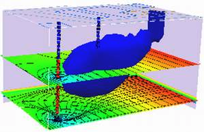
10. Analytical Solutions (2D)#
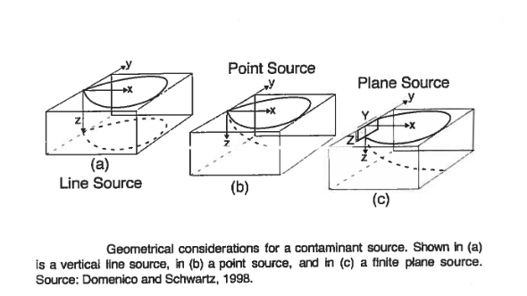
Domenico and Robbins (1985) conjectured that orthogonal (1D) solutions could be combined using superposition (and convolution) to create approximations to 2D and 3D behavior for simple, but useful geometries such as
Course Website
%%html
<style> table {margin-left: 0 !important;} </style>
Readings#
Hunt, B. (1978) Dispersive sources in uniform ground water flow. Journal of the Hydraulics Division, 104 (HY1), 75-85.
Videos#
The Domenico-Robbins (1985) solution is a heuristic simplification of an analytical solution to the advection-dispersion equation with sorption and reaction terms that can be programmed into spreadsheets or scripting environments without a full commitment to learning … The simplification comes with advantages that make it a reasonable alternative to exact solutions for simulations representative of many realistic scenarios.
Applications and Significance#
The 2D/3D Domenico solutions have been widely used by regulators, practitioners, and researchers due its ease of use and analytical origin. However, the lack of mathematical rigor in its derivation has raised questions about its accuracy with differing conclusions about its suitability for continued use.
It has been used as a regulatory tool as recently as 2014 (e.g. User’s Manual for the Quick Domenico Groundwater Fate-and-Transport Model (2014) Pensylvania Department of Environmental Protection).
Its significance lies in its ability to provide a rapid approximation of groundwater contamination scenarios, allowing for improved decision-making and risk assessment. As already stated there is criticism that the Domenico solution is unsuitable for use in professional and research applications because of departures from exact solutions under certain conditions.
Note
Given that all models are approximations its kind of a sorry critique. If you are modeling for real money, it would be prudent to apply multiple tools and not make decisions using only these analytical solutions.
… there is no need to ask ‘is the model true?’ The answer is ‘No.’ The only question of interest is ‘Is the model illuminating and useful?’ (Box, 1979 )
It is worth noting that the strongest argument against use of the Domenico solution is that modern computers and readily available $oftware can provide users with exact solutions or well established numerical models so there is no justification for using anything less. This position has some merit where decisions of weight with financial or environmental consequences depend on the modeling result.
As a side note readily available $oftware is NOT easy to install and use; the graphical interfaces tend to tied to specific architecture (x86-64) and specific operating systems. Hence availability does not imply the tools will get used - these simplified models still have value and will for a long time.
Yuan (1995) examined the “mathematical rigor” and provides detailed derivations of various solutions using convolution of elementry solutions (Carslaw and Jaeger 1959). While not at all resolving the critique, it provides interested readers with background and insight into the Domenico solution approximation(s).
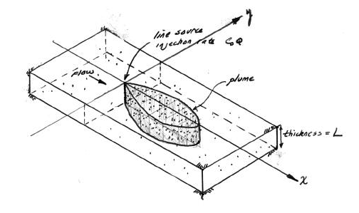
2D - Advection-Dispersion, Finite-Width, Constant Source#
Note
This is one of several Domenico-based multi-dimension solutions. More will be added as time permits. Bear in mind that spatial convolution can be applied for constructing different source geometries, as can convolution (superposition in time) for different input histories.
The sketch depicts a finite-length horizontal line source (complete mixing in \(z\) is assumed - i.e. no verticial variation) in an aquifer of infinite extent located at \((x,y)=(0,0)\). The length of the source zone (line) is \(Y\).
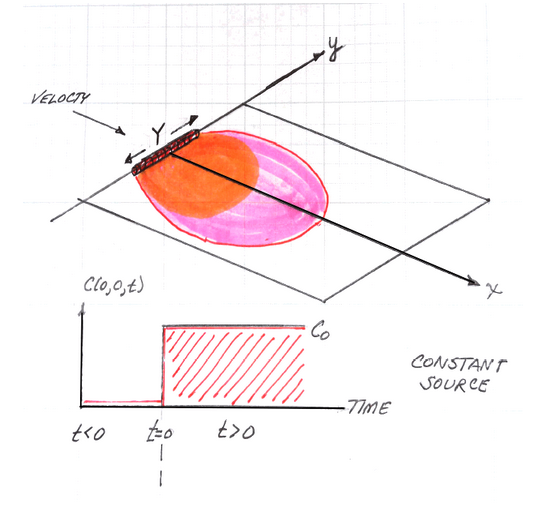
The source history is depicted beneath the sketch. The system starts with initial concentration of zero everywhere, at time \(t=0\), the concentration in the source line increases to \(C_0\) suddenly, and is maintained at that value from then on.
The transport processes modeled are advection along the x-axis, and dispersion in the x-direction (longitudinal) and in the y-direction (transverse).
The analytical model (Domenico and Robbins, 1985) was obtained by convolution of instantaneous sources (described in detail in Yuan, 1995):
A prototype function is
# prototype 2D domenico robbins ADE function
def c2ad(conc0, distx, disty, dispx, dispy, velocity, time, lenY):
    import math
    from scipy.special import erf, erfc # scipy needs to already be loaded into the kernel
    vadj = velocity / 1.0 # structure is in anticipation of adding adsorbtion and decay
    dispXadj = dispx / 1.0
    dispYadj = dispy / 1.0
    lambadj = 0 / 1.0

    uuu = math.sqrt(1.0 + 4.0*lambadj*dispXadj/vadj)
    ypp = (disty + 0.5*lenY) / (2*math.sqrt(dispYadj*distx))
    ymm = (disty - 0.5*lenY) / (2*math.sqrt(dispYadj*distx))

    arg1 = (distx - vadj*time*uuu) / (2*math.sqrt(dispXadj*vadj*time))
    arg2 = (distx / (2*dispXadj)) * (1 - uuu)

    term0 = conc0 / 4
    term1 = math.exp(arg2)
    term2 = erfc(arg1)
    term3 = (erf(ypp) - erf(ymm))

    c2ad = term0 * term1 * term2 * term3
    return c2ad
Supply model conditions, evaluate specific point in space and time.
# inputs
c_initial = 100.0 # g/m^3
xx = 100 # meters
yy = 0 # meters
Dx = 0.50 # m^2/day
Dy = 0.05 # m^2/day
V = 1.0 # m/day
time = 100.0 # days
Y = 10.0 # meters
alphax = Dx/V
alphay = Dy/V
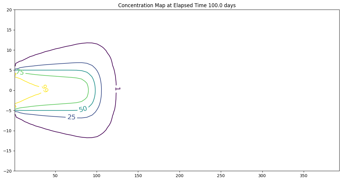
output=c2ad(c_initial, xx, yy, alphax, alphay, V, time, Y)
print("x= ",round(xx,2)," y= ",round(yy,2)," t= ",round(time,1)," C(x,y,t) = ",round(output,3))
x= 100 y= 0 t= 100.0 C(x,y,t) = 44.308
Construct 2D contour plots (equivalent to a profile plot)
# make a plot
x_max = 400
y_max = 20
# build a grid
nrows = 50
deltax = (x_max)/nrows
x = []
x.append(1)
for i in range(nrows):
    if x[i] == 0.0:
        x[i] = 0.00001
    x.append(x[i]+deltax)

ncols = 50
deltay = (y_max*2)/(ncols-1)
y = []
y.append(-y_max)
for i in range(1,ncols):
    if y[i-1] == 0.0:
        y[i-1] = 0.00001
    y.append(y[i-1]+deltay)

#y

#y = [i*deltay for i in range(how_many_points)] # constructor notation
#y[0]=0.001
ccc = [[0 for i in range(nrows)] for j in range(ncols)]

for jcol in range(ncols):
    for irow in range(nrows):
        ccc[irow][jcol] = c2ad(c_initial, x[irow], y[jcol], alphax, alphay, V, time, Y)

#y

my_xyz = [] # empty list
count=0
for irow in range(nrows):
    for jcol in range(ncols):
        my_xyz.append([ x[irow],y[jcol],ccc[irow][jcol] ])
       # print(count)
        count=count+1

#print(len(my_xyz))

import pandas
my_xyz = pandas.DataFrame(my_xyz) # convert into a data frame
import numpy
import matplotlib.pyplot
from scipy.interpolate import griddata
# extract lists from the dataframe
coord_x = my_xyz[0].values.tolist() # column 0 of dataframe
coord_y = my_xyz[1].values.tolist() # column 1 of dataframe
coord_z = my_xyz[2].values.tolist() # column 2 of dataframe
#print(min(coord_x), max(coord_x)) # activate to examine the dataframe
#print(min(coord_y), max(coord_y))
coord_xy = numpy.column_stack((coord_x, coord_y))
# Set plotting range in original data units
lon = numpy.linspace(min(coord_x), max(coord_x), 64)
lat = numpy.linspace(min(coord_y), max(coord_y), 64)
X, Y = numpy.meshgrid(lon, lat)
# Grid the data; use linear interpolation (choices are nearest, linear, cubic)
Z = griddata(numpy.array(coord_xy), numpy.array(coord_z), (X, Y), method='cubic')
# Build the map
fig, ax = matplotlib.pyplot.subplots()
fig.set_size_inches(14, 7)
CS = ax.contour(X, Y, Z, levels = [1,25,50,75,99])
ax.clabel(CS, inline=1, fontsize=16)
ax.set_title('Concentration Map at Elapsed Time '+ str(round(time,1))+' days');
Evaluate specific points
2D - Advection-Dispersion, Finite-Width, Finite-Duration Source#
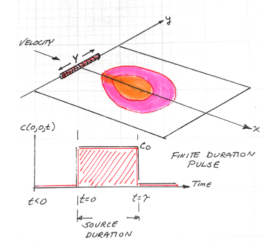
The sketch depicts a finite-length horizontal line source in an aquifer of infinite extent located at \((x,y)=(0,0)\) (again no variation in the \(z\) direction). The length of the source zone (line) is Y. The source history is depicted beneath the sketch. The system starts with initial concentration of zero everywhere, at time \(t=0\), the concentration in the source line increases to \(C_0\) suddenly, and is maintained at that value for a specified duration (\(\tau\)), when the source then decreases back to zero.
An analytical model based on Domenico and Robbins (1985) was obtained by convolution (temporal superposition) of two continuous sources shifted in time relative to one another, with the later source having opposite sense (sign) (This particular solution is described in detail in Yuan, 1995):
A prototype function is constructed from c2ad as follows:
# prototype 2D domenico robbins ADE function
def c2adfd(conc0, distx, disty, dispx, dispy, velocity, time, lenY, tau):
    import math
    from scipy.special import erf, erfc # scipy needs to already be loaded into the kernel
# internal definition of ordinary c2ad function ########################
    def c2ad(conc0, distx, disty, dispx, dispy, velocity, time, lenY):

        vadj = velocity / 1.0 # structure is in anticipation of adding adsorbtion and decay
        dispXadj = dispx / 1.0
        dispYadj = dispy / 1.0
        lambadj = 0 / 1.0

        uuu = math.sqrt(1.0 + 4.0*lambadj*dispXadj/vadj)
        ypp = (disty + 0.5*lenY) / (2*math.sqrt(dispYadj*distx))
        ymm = (disty - 0.5*lenY) / (2*math.sqrt(dispYadj*distx))

        arg1 = (distx - vadj*time*uuu) / (2*math.sqrt(dispXadj*vadj*time))
        arg2 = (distx / (2*dispXadj)) * (1 - uuu)

        term0 = conc0 / 4
        term1 = math.exp(arg2)
        term2 = erfc(arg1)
        term3 = (erf(ypp) - erf(ymm))

        c2ad = term0 * term1 * term2 * term3
        return c2ad
#########################################################################
    part1 = c2ad(conc0, distx, disty, dispx, dispy, velocity, time, lenY)
    part2 = c2ad(conc0, distx, disty, dispx, dispy, velocity, time-tau , lenY) #time-shift here
    c2adfd = part1-part2
    return c2adfd
Supply model conditions, evaluate specific point in space and time.
# inputs
c_initial = 100.0 # g/m^3
xx = 75 # meters
yy = 0 # meters
Dx = 0.50 # m^2/day
Dy = 0.05 # m^2/day
V = 1.0 # m/day
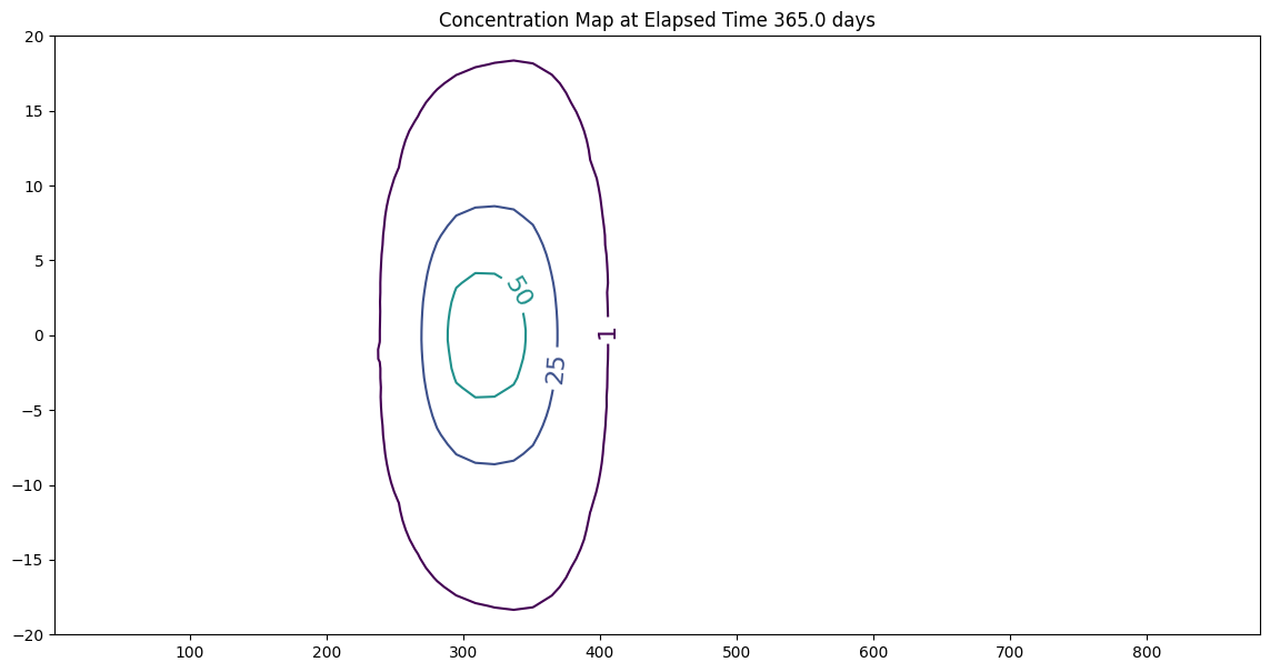
time = 365.0 # days
tau = 90.0 # days
Y = 10.0 # meters
alphax = Dx/V
alphay = Dy/V
output=c2adfd(c_initial, xx, yy, alphax, alphay, V, time, Y, tau)
print("x= ",round(xx,2)," y= ",round(yy,2)," t= ",round(time,1)," C(x,y,t) = ",round(output,3))
x= 75 y= 0 t= 365.0 C(x,y,t) = 0.0
Construct 2D contour plots (equivalent to a profile plot)
# make a plot
x_max = 900
y_max = 20
# build a grid
nrows = 50
deltax = (x_max)/nrows
x = []
x.append(1)
for i in range(nrows):
    if x[i] == 0.0:
        x[i] = 0.00001
    x.append(x[i]+deltax)

ncols = 50
deltay = (y_max*2)/(ncols-1)
y = []
y.append(-y_max)
for i in range(1,ncols):
    if y[i-1] == 0.0:
        y[i-1] = 0.00001
    y.append(y[i-1]+deltay)

#y

#y = [i*deltay for i in range(how_many_points)] # constructor notation
#y[0]=0.001
ccc = [[0 for i in range(nrows)] for j in range(ncols)]

for jcol in range(ncols):
    for irow in range(nrows):
        ccc[irow][jcol] = c2adfd(c_initial, x[irow], y[jcol], alphax, alphay, V, time, Y, tau)

#y

my_xyz = [] # empty list
count=0
for irow in range(nrows):
    for jcol in range(ncols):
        my_xyz.append([ x[irow],y[jcol],ccc[irow][jcol] ])
       # print(count)
        count=count+1

#print(len(my_xyz))

import pandas
my_xyz = pandas.DataFrame(my_xyz) # convert into a data frame
import numpy
import matplotlib.pyplot
from scipy.interpolate import griddata
# extract lists from the dataframe
coord_x = my_xyz[0].values.tolist() # column 0 of dataframe
coord_y = my_xyz[1].values.tolist() # column 1 of dataframe
coord_z = my_xyz[2].values.tolist() # column 2 of dataframe
#print(min(coord_x), max(coord_x)) # activate to examine the dataframe
#print(min(coord_y), max(coord_y))
coord_xy = numpy.column_stack((coord_x, coord_y))
# Set plotting range in original data units
lon = numpy.linspace(min(coord_x), max(coord_x), 64)
lat = numpy.linspace(min(coord_y), max(coord_y), 64)
X, Y = numpy.meshgrid(lon, lat)
# Grid the data; use linear interpolation (choices are nearest, linear, cubic)
Z = griddata(numpy.array(coord_xy), numpy.array(coord_z), (X, Y), method='cubic')
# Build the map
fig, ax = matplotlib.pyplot.subplots()
fig.set_size_inches(14, 7)
CS = ax.contour(X, Y, Z, levels = [1,25,50,75,99])
ax.clabel(CS, inline=1, fontsize=16)
ax.set_title('Concentration Map at Elapsed Time '+ str(round(time,1))+' days');
2D Plume in Regional Flow (Hunt Solution)#
The sketch depicts a vertical line source in an aquifer of infinite extent located at (x,y)=(0,0) some time after constant injection has begun.
For the line source (injection well) whose fluid contribution makes negligible impact on the local hydraulics as depicted in the sketch the initial, boundary, and mass conservation conditions are:
A solution obtained by time-convolution of an elementary line source solution (Hunt, 1978) is
where \(W(a,b)\) is the leaky aquifer (Hantush) well function with
The solution is presented in (Bear, 1972) as a convolution integral (eqn. 10.6.38, p. 634) (the end user needs to supply the integration routine); Hunt (1978) noticed that the integral was the leaky well function with appropriate substitutions and completed the solution.
The leaky aquifer function can be evaluated numerically using a recursive definition, or efficient approximations can be used. Listings for these approximations appear below after the references
The solution is applicable for porous media flow, where the velocity (below) is the mean section velocity (seepage velocity divided by the porosity). The solution can also be used with streams and pipes (porosity = 1). Negative values of distance in x-axis would correspond to locations upgradient of the injection location.
Scripts to generate solutions are listed below:
Leaky Well Function#
def wh(u, rho): # Hantush Leaky aquifer well function
    import numpy
    """Returns Hantush's well function values

    Note: works only for scalar values of u and rho

    Parameters:
    -----------
    u : scalar  (u= r^2 * S / (4 * kD * t))
    rho : sclaar (rho =r / lambda, lambda = sqrt(kD * c))
    Returns:
    --------
    Wh(u, rho) : Hantush well function value for (u, rho)
    """
    try:
        u =float(u)
        rho =float(rho)
    except:
        print("u and rho must be scalars.")
        raise ValueError()

    LOGINF = 2
    y = numpy.logspace(numpy.log10(u), LOGINF, 1000)
    ym = 0.5 * (y[:-1]+  y[1:])
    dy = numpy.diff(y)
    wh = numpy.sum(numpy.exp(-ym - (rho / 2)**2 / ym ) * dy / ym)
    return(wh)
Hunt Solution (Prototype Function)#
def chunt(c_injection,q_injection,l_thickness,d_x,d_y,velocity,x_location,y_location,time):
    import math
    rsq = (x_location**2 + (y_location**2)*(d_x/d_y))
    rrr = math.sqrt(rsq)
    aaa = rsq/(4.0*d_x*time)
    bbb = (rrr*velocity)/(2.0*d_x)
#    print(rsq,rrr,aaa,bbb)
    term1 = c_injection*q_injection/(4.0*math.pi*l_thickness)
    term2 = 1.0/(math.sqrt(d_x*d_y))
    term3 = math.exp((x_location*velocity)/(2.0*d_x))
#    term4 = leakyfn(aaa,bbb)
    term4 = wh(aaa,bbb)

    #if term4 <= 0.0: term4 = 0.0
#    print(term1,term2,term3,term4)
    chunt = term1*term2*term3*term4
    return chunt
Driver Script#
# inputs
c_injection = 133
q_injection = 3.66
l_thickness = 1.75
d_x = 0.920
d_y = 0.092
velocity = 0.187
x_location = 123
y_location = 0
time = 36500
scale = c_injection*q_injection
output = chunt(c_injection,q_injection,l_thickness,d_x,d_y,velocity,x_location,y_location,time)
print("Concentration at x = ",round(x_location,2)," y= ",round(y_location,2) ," t= ",round(time,2) ," = ",round(output,3))
#
Concentration at x = 123 y= 0 t= 36500 = 53.424
Plotting Script#
# make a plot
x_max = 200
y_max = 100
# build a grid
nrows = 50
deltax = (x_max*4)/nrows
x = []
x.append(-x_max)
for i in range(nrows):
    if x[i] == 0.0:
        x[i] = 0.00001
    x.append(x[i]+deltax)

ncols = 50
deltay = (y_max*2)/(ncols-1)
y = []
y.append(-y_max)
for i in range(1,ncols):
    if y[i-1] == 0.0:
        y[i-1] = 0.00001
    y.append(y[i-1]+deltay)

#y

#y = [i*deltay for i in range(how_many_points)] # constructor notation
#y[0]=0.001
ccc = [[0 for i in range(nrows)] for j in range(ncols)]

for jcol in range(ncols):
    for irow in range(nrows):
        ccc[irow][jcol] = chunt(c_injection,q_injection,l_thickness,d_x,d_y,velocity,x[irow],y[jcol],time)

#y

my_xyz = [] # empty list
count=0
for irow in range(nrows):
    for jcol in range(ncols):
        my_xyz.append([ x[irow],y[jcol],ccc[irow][jcol] ])
       # print(count)
        count=count+1

#print(len(my_xyz))

import pandas
my_xyz = pandas.DataFrame(my_xyz) # convert into a data frame
import numpy
import matplotlib.pyplot
from scipy.interpolate import griddata
# extract lists from the dataframe
coord_x = my_xyz[0].values.tolist() # column 0 of dataframe
coord_y = my_xyz[1].values.tolist() # column 1 of dataframe
coord_z = my_xyz[2].values.tolist() # column 2 of dataframe
#print(min(coord_x), max(coord_x)) # activate to examine the dataframe
#print(min(coord_y), max(coord_y))
coord_xy = numpy.column_stack((coord_x, coord_y))
# Set plotting range in original data units
lon = numpy.linspace(min(coord_x), max(coord_x), 64)
lat = numpy.linspace(min(coord_y), max(coord_y), 64)
X, Y = numpy.meshgrid(lon, lat)
# Grid the data; use linear interpolation (choices are nearest, linear, cubic)
Z = griddata(numpy.array(coord_xy), numpy.array(coord_z), (X, Y), method='cubic')
# Build the map
fig, ax = matplotlib.pyplot.subplots()
fig.set_size_inches(10, 5)
CS = ax.contour(X, Y, Z, levels = [1,5,10,15,20,25,30,35,40,45,50])
ax.clabel(CS, inline=2, fontsize=16)
ax.set_title('Concentration Map at Elapsed Time '+ str(round(time,1))+' days');

Spreadsheet Model#
A spreadsheet implementation is available at http://54.243.252.9/ce-5364-webroot/6-Spreadsheets/HuntModel.xlsm
Note
This model requires Analysis Tool Pack Add-In and the VBA Macro Enabled. May no longer work in current cloud-based Excel
Useful Code Listings#
Polynomial Approximation
The approximations below are coded in python, and can convert to spreadsheet using VBA fairly easily. These are based on polynomial approximations in:
Abramowitz, M. and I.A. Stegun, 1964. Handbook of Mathematical Functions with Formulas, Graphs, and Mathematical Tables. U.S. Department of Commerce, National Bureau of Standards, Applied Mathematics Series, Vol 55.
And seem to produce nearly the same results as the recursive version above.
#######################
# Theis Well Function #
#######################
def wellfn(u):
    import math
    if ((u >= 0) and (u <=1)):
# polynomial approximation constants
        a0 = -0.57721566
        a1 =  0.99999193
        a2 = -0.24991055
        a3 =  0.05519968
        a4 = -0.00976004
        a5 =  0.00107857
        wellfn = -math.log(u) + a0 + a1*u + a2*u**2 + a3*u**3 + a4*u**4 + a5*u**5
        return(wellfn)
    elif ((u >1)):
# polynomial approximation constants
        a1 =  8.5733287401
        a2 = 18.0590169730
        a3 =  8.6347608925
        a4 =  0.2677737343
        b1 =  9.5733223454
        b2 = 25.6329561486
        b3 = 21.0996530827
        b4 =  3.9584969228
        frac1 = u**4 + a1*u**3 + a2*u**2 + a3*u + a4
        frac2 = u**4 + b1*u**3 + b2*u**2 + b3*u + b4
        frac3 = u*math.exp(u)
        wellfn = (frac1/frac2)/frac3
        return(wellfn)
    else:
        print('error in wellfn')
        wellfn = -999.0
        return(wellfn)

#######################
# Leaky Well Function #
#######################
def leakyfn(u,v):
    import math
    import numpy
    from scipy.special import kn as besselK
    from scipy.special import iv as besselI
# finite series recursion constants
    c12 =  0.0277777777777778
#
    c14 = -0.00347222222222222
    c15 =  0.00173611111111111
#
    c17 =  0.000416666666666667
    c18 = -0.000138888888888889
    c19 =  0.0000694444444444444
#
    c21 = -0.0000462962962962963
    c22 =  0.0000115740740740741
    c23 = -3.85802469135802E-06
    c24 =  1.92901234567901E-06
#
    c26 =  4.72411186696901E-06
    c27 = -9.44822373393802E-07
    c28 =  2.3620559334845E-07
    c29 = -7.87351977828168E-08
    c30 =  3.93675988914084E-08
#
    c32 = -4.42885487528345E-07
    c33 =  7.38142479213908E-08
    c34 = -1.47628495842782E-08
    c35 =  3.69071239606954E-09
    c36 = -1.23023746535651E-09
    c37 =  6.15118732678257E-10
#
# entry point
    a3 = (v**2)/4
# if leakance term is negligible, then return well function
    if (a3 == 0) :
        leakyfn = wellfn(u)
        return(leakyfn)
# if leakance/time term is large enough, then return besselKo
    if (a3/u > 5) :
        leakyfn = 2*besselK(0,v)
        return(leakyfn)
#  }
# finite series approximation for u>1, v<=2
    if ((u >= 1) and (v <= 2)) :
    # recursion terms built by-hand (ported from SSANTS)
        g11 = c12*a3
        g12 = c14*(a3**2)/(u)
        g21 = c15*(a3**2)
        g22 = c17*(a3**3)/(u**2)
        g23 = c18*(a3**3)/(u)
        g31 = c19*(a3**3)
        g32 = c21*(a3**4)/(u**3)
        g33 = c22*(a3**4)/(u**2)
        g34 = c23*(a3**4)/(u)
        g41 = c24*(a3**4)
        g42 = c26*(a3**5)/(u**4)
        g43 = c27*(a3**5)/(u**3)
        g44 = c28*(a3**5)/(u**2)
        g45 = c29*(a3**5)/(u)
        g51 = c30*(a3**5)
        g52 = c32*(a3**6)/(u**5)
        g53 = c33*(a3**6)/(u**4)
        g54 = c34*(a3**6)/(u**3)
        g55 = c35*(a3**6)/(u**2)
        g56 = c36*(a3**6)/(u)
        g61 = c37*(a3**6)
    # sum them up!
        a34list = [g11,g12,g21,g22,g23,g31,g32,g33,g34,g41,g42,g43,g44,g45,g51,g52,g53,g54,g55,g56,g61]
        a34 = numpy.sum(a34list)
        a35 = a34*math.exp(-u)
        a36 = a3/u
        a37 = besselI(v,0)
        a38 = wellfn(u)*a37
        a39 = 0.5772 + math.log(a36) + wellfn(a36) - a36 +(besselI(0,v)-1)/u
        a40 = a39*math.exp(-u)
        leakyfn = a38 - a40 + a35
        leakyfn=abs(leakyfn)
        return(leakyfn)
# finite series approximation for u<=1, v<=2
    if ((u <= 1) and (v <= 2)) :
    # recursion terms built by-hand (ported from SSANTS)
        g11 = c12*a3
        g12 = c14*(a3)/(u**-1)
        g21 = c15*(a3**2)
        g22 = c17*(a3)/(u**-2)
        g23 = c18*(a3**2)/(u**-1)
        g31 = c19*(a3**3)
        g32 = c21*(a3)/(u**-3)
        g33 = c22*(a3**2)/(u**-2)
        g34 = c23*(a3)/(u**-1)
        g41 = c24*(a3**4)
        g42 = c26*(a3)/(u**-4)
        g43 = c27*(a3**2)/(u**-3)
        g44 = c28*(a3**3)/(u**-2)
        g45 = c29*(a3**4)/(u**-1)
        g51 = c30*(a3**5)
        g52 = c32*(a3)/(u**-5)
        g53 = c33*(a3**2)/(u**-4)
        g54 = c34*(a3**3)/(u**-3)
        g55 = c35*(a3**4)/(u**-2)
        g56 = c36*(a3**5)/(u**-1)
        g61 = c37*(a3**6)
    # sum them up!
        a70list = [g11,g12,g21,g22,g23,g31,g32,g33,g34,g41,g42,g43,g44,g45,g51,g52,g53,g54,g55,g56,g61]
        a70 = numpy.sum(a70list)
        a71 = u*a70
        a72 = a3/u
        a73 = 0.5772+math.log(u)+wellfn(u)-u+(besselI(0,v)-1)/(a72)
        a74 = a73*math.exp(-a72)
        a75 = besselI(0,v)*wellfn(a72)
        a76 = a75 - a74 + a71
        a77 = 2*besselK(0,v)
        leakyfn = (a77-a76)
        return(leakyfn)
# approximation for v > 2
    if (v > 2) :
        term1 = math.sqrt(pi/(2*v))
        term2 = math.exp(-v)
        term3 = -(v-2*u)/(2*math.sqrt(u))
        term4 = math.erfc(term3)
        leakyfn = term1*term2*term4
        return(leakyfn)
    else:
        print('error in leakyfn')
        leakyfn = -999.0
        return(leakyfn)
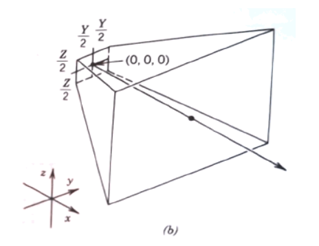
3D - Advection-Dispersion, Finite-Area, Constant Production (Injection) Source#
The sketch depicts a planar source zone Y units wide and Z units tall, centered at (0,0,0).
The analytical model (Domenico and Robbins, 1985) is obtained by convolution of instantaneous sources (described in detail in Yuan, 1995):
Note
This solution is identical to Equation 6.33, with \(\lambda = 0\), \(R = 1\).
A prototype function is
def c3dad(conc0, distx, disty, distz, lenX, lenY, lenZ, dispx, dispy, dispz, velocity, etime):
    import math
    from scipy.special import erf, erfc # scipy needs to already be loaded into the kernel
    # Constant of integration
    term1 = conc0 / 8.0

    # Centerline axis solution
    arg1 = (distx - velocity*etime) / (2*math.sqrt(dispx*velocity*etime)) #dispx is dispersivity
    term2 = erfc(arg1)

    # Off-axis solution, Y direction
#    arg2 = 2.0 * math.sqrt(dispy*distx / velocity)
    arg2 = 2.0 * math.sqrt(dispy*distx) #dispy is dispersivity
    arg3 = disty + 0.5*lenY
    arg4 = disty - 0.5*lenY
    term3 = erf(arg3 / arg2) - erf(arg4 / arg2)

    # Off-axis solution, Z direction
#    arg5 = 2.0 * math.sqrt(dispz*distx / velocity)
    arg5 = 2.0 * math.sqrt(dispz*distx) #dispz is dispersivity
    arg6 = distz + 0.5*lenZ
    arg7 = distz - 0.5*lenZ
    term4 = erf(arg6 / arg5) - erf(arg7 / arg5)

    # Convolve the solutions
    c3dad = term1 * term2 * term3 * term4
    return c3dad
Warning
The is 3D code is incomplete. Needs
An example
Refactor to enforce best code practices
Script to render an xyz density plot
Exercise(s)#
# autobuild exercise
import subprocess

try:
    subprocess.run(["pdflatex", "ce5364-es5-2025-3.tex"],
                   stdout=subprocess.DEVNULL, stderr=subprocess.DEVNULL, check=True)
except subprocess.CalledProcessError:
    print("Build failed. Check your LaTeX source file.")