
3. Infiltration, Evaporation, and Soil Moisture#
Course Website
Readings#
Chow, V.T., Maidment, D.R., Mays, L.W., 1988, Applied Hydrology: New York, McGraw-Hill. pp. 80-91
Gupta, R.S., 2017. Hydrology and Hydraulic Systems, pp. 65-88; pp. 93-111
Chow, V. T., 1964. Handbook of Applied Hydrology. McGraw Hill, New York. Sec. 14., 2pp.
Wurbs and James, 2002. Water Resources Engineering. Prentice-Hall, New Jersey. Pp 462-483.
Polubarinova-Kochina, 1962. Theory of Groundwater Movement, (Translated from Russian by R. De Wiest), Princeton University Press, New Jersey.
VICAIRE (VIrtual CAmpus In hydrology and water REsources management) Used as source for some images, and instructional content.
Spreadsheets#
Green-Ampt Spreadsheet (Excel) Right-Click “Save As…”
Blaney-Criddle Spreadsheet (Excel) Right-Click “Save As…”
Thornwaithe Spreadsheet (Excel) Right-Click “Save As…”
Videos#
This section, while titled Infiltration, Evaporation, and Soil Moisture, is broadly concerned with the concept of hydrologic abstractions—the collection of processes that divert water from contributing to surface runoff. These abstractions include infiltration into the soil, evaporation from land and water surfaces, transpiration from vegetation, interception by canopy and surface storage, and temporary retention in depressions or surface roughness. Each of these processes removes a portion of the precipitation before it can contribute to streamflow. The difference between the incoming precipitation and the total abstraction defines the runoff available for routing through a watershed. Understanding these processes is critical for modeling rainfall-runoff behavior, estimating water availability, and managing both flood risk and drought resilience.
Infiltration Process and Factors Affecting It#
One of the key factors affecting how much rainfall becomes runoff in a watershed is infiltration; the process by which water enters the soil. This is part of what we call hydrologic abstractions, which are the various ways water is absorbed, retained, or evaporated before it ever contributes to surface flow. In simple terms, the water that doesn’t run off is either infiltrating into the ground or returning to the atmosphere in some form.
The amount of runoff we ultimately see is the difference between the rainfall that falls and the portion that is removed by these abstraction processes. Importantly, soil moisture conditions at the time of the storm play a major role. If the soil is already saturated, much less water will infiltrate—leading to more runoff. Conversely, dry soils can absorb a greater amount of water, reducing surface flow. So when we’re modeling stormwater or flood behavior, it’s critical that we account for how infiltration and soil moisture interact over time.
Infiltration is a complex process influenced by multiple factors such as soil characteristics, land use, slope, vegetation cover, precipitation intensity, and human activities. The soil’s permeability, texture, structure, and moisture content significantly impact infiltration rates. Coarse soils with higher permeability tend to have higher infiltration rates compared to fine-textured soils like clay. Importance and Roles:
Roles in hydrology:#
Water Availability: Infiltration governs the replenishment of groundwater resources, contributing to the sustained flow of streams and rivers during dry periods. A high infiltration rate allows water to percolate deeper into the soil, recharging aquifers and maintaining base flow in rivers.
Flood Mitigation: Adequate infiltration helps prevent surface runoff, reducing the risk of flooding by allowing water to infiltrate into the soil, thus delaying the onset of overland flow.
Water Quality: Infiltration acts as a natural filter, removing pollutants and impurities as water percolates through the soil. However, excessive or improper land use can compromise this filtration capacity, leading to contamination of surface water resources.
Factors Affecting Infiltration Processes:#
Land Use: Urbanization and deforestation can reduce natural infiltration rates due to increased impervious surfaces, resulting in enhanced surface runoff and decreased groundwater recharge.
Climate Change: Alterations in precipitation patterns and intensities due to climate change can affect infiltration rates, potentially leading to soil erosion and reduced water infiltration capacities.
Soil Management Practices: Techniques such as cover cropping, no-till agriculture, and contour plowing can help enhance soil structure and organic matter, promoting better infiltration.
Engineering Enhancement Strategies:#
Green Infrastructure: Implementing green spaces, permeable pavements, and rain gardens in urban areas can enhance infiltration rates and decrease surface runoff.
Soil Conservation: Practices like terracing, contour farming, and agroforestry aid in reducing soil erosion, enhancing soil structure, and preserving natural infiltration capacities.
Education and Regulation: Public awareness campaigns and policies regarding responsible land use and water management can aid in preserving natural infiltration processes.
3.1 Infiltration Models#
Examination of various process models at
Infiltration Process Description#
Water that soaks into the ground and thereby enters the soil structure is considered removed from the runoff process at the time it enters the soil. The process by which this occurs is called infiltration. This process is the first step in a lengthy and vital process, the interaction of soil, water, air, and plant life.
The soil matrix in its simplest form consists of particles of soil (minerals) loosely packed together in such a way that there are void spaces (pores). The pores are filled by either air or by water. If the voids are completely filled with water, the soil is said to be saturated. If a volume of saturated soil overlies something that does not block flow, some of the water contained in it will drain away, and some will remain trapped in the pore spaces in the soil by capillary forces. The size of the pore spaces in natural soils is such that capillary forces are important in the movement of water through them. The amount of water that drains through is called gravitational water, and is particular to the soil, as is the amount retained. The water retained balances forces between gravity and capillarity, and maintains equilibrium.
Plants have roots that penetrate the upper soil layers, and remove water held there by cap-illarity. The upper layers of soil are thereby unbalanced, having capillary potential available to take up water. When rain falls on such a soil, there are initially two forces driving water into the soil- gravity and capillarity. If sufficient rain is available, the upper layers of the soil will become saturated, and the water will proceed downward. Due to the dual forces of capillarity and gravity, the initial rate of uptake of water may be quite high. As the capillary force is satisfied, gravity becomes the only force and the rate of uptake reaches an equilibrium value, as gravitational water drains through the soil.
The progress of this phenomenon can be shown graphically sketch on board. Initially, the rate of infiltration is quite high, and it decays to a steady-state value as a first-order function of time.
Mathematically, there have been a number of relationships proposed to represent this progress. Collectively these equations represent different loss models. They are all attempts to explain a complex phenomenon currently beyond our understanding at any but the smallest scales. What follows are the set of more common models in use.
Proportional Loss Model#
The loss is some proportion of the incoming rainfall. Somewhat similar in mindset to the rational method, but every rainfall pulse produces runoff (albeit possibly quite small). It does produce good mass balance with observations.
[NEED TO COMPLETE SECTION]
Horton’s Model#
Hortons equation is one of the simpler, and is presented here:
where \(q(t)\) = the infiltration rate at time \(t\), in length/time;
\(f_c\) = the equilibrium infiltration rate, in length/time;
\(f_o\) = the initial infiltration rate, in length/time;
\(k\) = a decay constant, particular to the soil, in reciprical time;
\(t\) = time.
The integral of Hortons equation with time is the volume of rainfall that infiltrates during an event.
where I(t) is cumulative infiltration at time t, a depth. The parameters in Hortons equation can be determined for any give soil by infiltrometer tests. The parameters in Hortons equation can be determined for any give soil by infiltrometer tests. A script to generate a graph of Hortons equation for \(f_c = 0.53~in/hr\), \(f_o = 3~in/hr\), and \(k = 4.182~hr^{−1}\) is listed below.
In the script below the input precipitation is set to slightly exceed the initial rate so that runoff is generated immediately, its mostly to show a runoff plot but is ancillary to the example.
## Hortonian Infiltration Excess Model
import math
howmany = 1000
k = 4.182 # watershed infiltration excess decay constant
f0 = 3.0 # initial infiltration rate
fC = 0.53 # asymptotic infiltration rate
#
pRate = 3.0001 # some constant rate in excess of fC, for plotting only!
Tend = 5.0 # rainfall duration

def qfunc(f0,fC,kay,time):
    qfunc = fC+(f0 - fC)*math.exp(-time*kay)
    return(qfunc)

def peein(rate,time,tend): # a simple hyetograph model
    if time >= tend:
        peein=0.0
    else:
        peein=rate
    return(peein)

qnow = [0 for i in range(howmany)]
CumQnow = [0 for i in range(howmany)]
CumPnow = [0 for i in range(howmany)]
PXSnow = [0 for i in range(howmany)]
time = [0 for i in range(howmany)]
deltat = 0.004 # time step value
# time zero values
qnow[0]=qfunc(f0,fC,k,time[0])
for itime in range(1,howmany):
    time[itime] = deltat+time[itime-1]
    qnow[itime]=qfunc(f0,fC,k,time[itime])
    CumQnow[itime]=qnow[itime]*deltat + CumQnow[itime-1]
 #   rnow[itime]=alpha*qfunc(peein,time[itime],alpha)
    PXSnow[itime]=peein(pRate,time[itime],Tend)*time[itime]-CumQnow[itime]
    CumPnow[itime]=peein(pRate,time[itime],Tend)*time[itime]

import matplotlib.pyplot # the python plotting library
myfigure = matplotlib.pyplot.figure(figsize = (10,5)) # generate a object from the figure class, set aspect ratio

# Built the plot
#matplotlib.pyplot.plot(pnow, pnow, color ='blue')
matplotlib.pyplot.plot(time, qnow, color ='orange')
matplotlib.pyplot.plot(time, CumQnow, color ='green')
matplotlib.pyplot.plot(time, PXSnow, color ='red')
matplotlib.pyplot.plot(time, CumPnow, color ='blue')
matplotlib.pyplot.ylim([0,2*max(qnow)])
matplotlib.pyplot.xlabel("Time (hours)")
matplotlib.pyplot.ylabel("Infiltration Rate (inches/hour) or Depth (inches)")
matplotlib.pyplot.title("Hortonian Infiltration Excess Model \n"+"F_initial ="+str(f0)+
                        " F_equilibrium ="+str(fC)+" Decay Constant (1/hr) ="+str(k) )
matplotlib.pyplot.legend(["Infiltration Rate (in/hr)","Infiltration Depth (inches)","Runoff Depth (inches)","Precipitation Depth (inches)"])
matplotlib.pyplot.show()
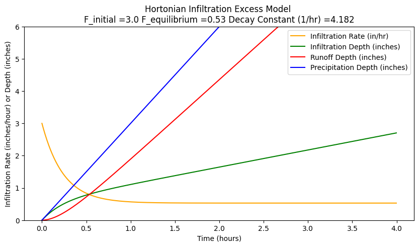
When rain begins, infiltration also begins, and is the initial value (denoted fo in Hortons equation) is quite high (in this case, \(3.0~in/hr\)). At that time, infiltration rate usually exceeds the intensity of rainfall. As the infiltration rate drops, it at some point intersects with the rate of rainfall. After that point, rainfall rate will exceed infiltration rate. With no runoff, water would begin to pond on the soil surface. The time from beginning of rain until that point is reached is called the time to ponding. After some time, the infiltration rate has dropped until it approaches an equilibrium value, represented by \(f_c\) (in this case, \(0.53~in/hr\)). After that time, gravity alone is the force driving the infiltration process.
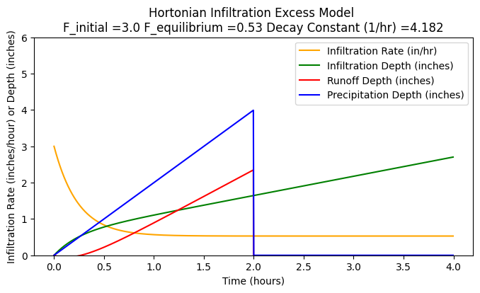
If the rainfall rate is less that the initial rate, and the storm duration is a bit shorter different results appear as below when the storm is shortened to 2 hours, and the rainfall rate is 2.0
## Hortonian Infiltration Excess Model
import math
howmany = 1000
k = 4.182 # watershed infiltration excess decay constant
f0 = 3.0 # initial infiltration rate
fC = 0.53 # asymptotic infiltration rate
#
pRate = 2.0001 # some constant rate in excess of fC, for plotting only!
Tend = 2.0 # rainfall duration

def qfunc(f0,fC,kay,time):
    qfunc = fC+(f0 - fC)*math.exp(-time*kay)
    return(qfunc)

def peein(rate,time,tend): # a simple hyetograph model
    if time >= tend:
        peein=0.0
    else:
        peein=rate
    return(peein)

qnow = [0 for i in range(howmany)]
CumQnow = [0 for i in range(howmany)]
CumPnow = [0 for i in range(howmany)]
PXSnow = [0 for i in range(howmany)]
time = [0 for i in range(howmany)]
deltat = 0.004 # time step value
# time zero values
qnow[0]=qfunc(f0,fC,k,time[0])
for itime in range(1,howmany):
    time[itime] = deltat+time[itime-1]
    qnow[itime]=qfunc(f0,fC,k,time[itime])
    CumQnow[itime]=qnow[itime]*deltat + CumQnow[itime-1]
 #   rnow[itime]=alpha*qfunc(peein,time[itime],alpha)
    PXSnow[itime]=peein(pRate,time[itime],Tend)*time[itime]-CumQnow[itime]
    CumPnow[itime]=peein(pRate,time[itime],Tend)*time[itime]

import matplotlib.pyplot # the python plotting library
myfigure = matplotlib.pyplot.figure(figsize = (8,4)) # generate a object from the figure class, set aspect ratio

# Built the plot
#matplotlib.pyplot.plot(pnow, pnow, color ='blue')
matplotlib.pyplot.plot(time, qnow, color ='orange')
matplotlib.pyplot.plot(time, CumQnow, color ='green')
matplotlib.pyplot.plot(time, PXSnow, color ='red')
matplotlib.pyplot.plot(time, CumPnow, color ='blue')
matplotlib.pyplot.ylim([0,2*max(qnow)])
matplotlib.pyplot.xlabel("Time (hours)")
matplotlib.pyplot.ylabel("Infiltration Rate (inches/hour) or Depth (inches)")
matplotlib.pyplot.title("Hortonian Infiltration Excess Model \n"+"F_initial ="+str(f0)+
                        " F_equilibrium ="+str(fC)+" Decay Constant (1/hr) ="+str(k) )
matplotlib.pyplot.legend(["Infiltration Rate (in/hr)","Infiltration Depth (inches)","Runoff Depth (inches)","Precipitation Depth (inches)"])
matplotlib.pyplot.show()
Phi-Index Infiltration Model#
The \(\phi\)-index is a simplified infiltration model commonly used in hydrology. It assumes that the infiltration capacity of the soil remains constant throughout a storm event, expressed as \(\phi\) (in/hr). When paired with observations from a rainfall hyetograph and runoff hydrograph, a suitable value for \(\phi\) can often be estimated with reasonable accuracy.
Field data indicate that infiltration capacity is highest at the onset of a storm and then decreases rapidly to a relatively stable value. Because this stabilization typically occurs within 10 to 15 minutes, it is generally acceptable to treat the infiltration rate as constant for the duration of the event.
The \(\phi\)-index approach simplifies hydrologic loss modeling as follows:
When rainfall intensity is less than the infiltration capacity, all rainfall infiltrates, and the loss rate equals the rainfall intensity.
When rainfall intensity exceeds the infiltration capacity, the loss rate is capped at \(\phi\).
This relationship is mathematically defined as:
where:
\(q(t)\) is the infiltration loss rate,
\(i(t)\) is the storm rainfall intensity at time \(t\),
\(\phi\) is the constant infiltration capacity.
To estimate \(\phi\) from measured rainfall-runoff data:
Separate baseflow from total runoff volume,
Compute the volume of direct runoff,
Determine the value of \(\phi\) such that the volume of effective rainfall (rainfall exceeding \(\phi\)) equals the volume of direct runoff.
Once individual storm values are computed, an average \(\phi\)-index may be derived to represent typical conditions for use in design and modeling.
Green-Ampt Model#
The Green-Ampt model is a simplified soil-physics model that is reasonably defendible in most hydrologic engineering situations.
The Green-Ampt model needs some soil mechanics context before presentation. The falling head permeameter is used when the hydraulic conductivity of the porous material is small. In this case, a constant head permeameter cannot easily generate a high enough gradient to produce measurable flow in a reasonable amount of time.
The figure below shows a schematic diagram of a falling head permeameter. A sample of porous medium is placed in the device. The length of the sample is \(L\), the cross-sectional area of the sample is \(A = \pi \frac{(2r_s)^2}{4}\). A smaller area tube rises above the sample with area \(a = \pi \frac{(2r)^2}{4} \). This tube provides the driving force required to move water through the porous sample with reasonably small water volume.
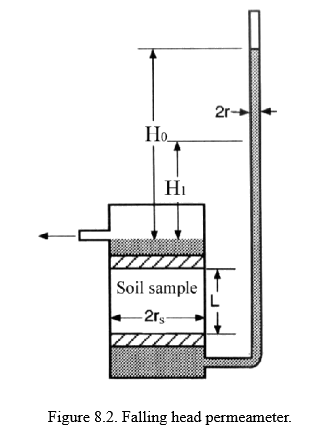
The head is measured at the inlet of the sample as the height of water in the tube above the sample, \(h(t)\). The flow rate through the sample is \(Q(t)\), and in a falling head permeameter, both \(h(t)\) and \(Q(t)\) vary with time.
Darcy’s law for this situation is:
A volume balance gives an alternate expression for discharge rate:
Separating variables and integrating:
Evaluating the integral gives:
This equation is linear in time, so a plot of \(\ln(h)\) versus time should yield a straight line. The slope is proportional to the hydraulic conductivity \(K\).
Now, turning to runoff and infiltration: in watershed settings, the tube and soil sample areas are essentially equal, but not all water infiltrates—some runs off after ponding.
Figure 4 illustrates infiltration over time. Water has infiltrated into the soil to depth \(z\) after some ponding. The amount infiltrated is:
The rate of wetting front movement is:
Darcy’s law from the surface to the wetting front is:
Equating the two rates gives:
Separate and integrate:
Using a partial fraction expansion:
Integration yields:
Setting \(t = 0\) and \(z = 0\) gives \(C = 0\). Rearranging:
Now define infiltration depth:
Substituting into the equation:
Classical Green-Ampt Form#
Green & Ampt (1911) simplified infiltration model is based on an approximation of the water content profile in a soil, as depicted in the figure below.
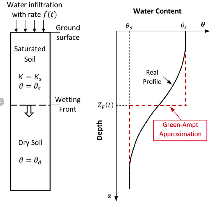
The wetting front is a sharp boundary (this sharp separation is the fundamental approximation) separating wet and dry soil zones. In Green-Ampt’s formulation the soil above the front is saturated, and that below is “dry.” The wetting front advances to depth \(L\) in time \(t\), with a small ponded depth \(h_0\) on the surface. The Green-Ampt equation is structurally similar to the derivation above, but with a new definition:
So the Green-Ampt formula becomes:
This expression gives the total cumulative infiltration at time \(t\) during a storm. Combined with rainfall data, it helps compute runoff by subtracting infiltration from total precipitation.
Green-Ampt is explicitly listed as the the preferred method in the TSARP report for Harris County. Many modeling tools (e.g., HEC-HMS, SWMM) support it using \(K\), \(\nabla \phi\), \(h_c\), and \(\psi_f\) forms.
My preference is to use the \(K\), \(n\), and \(h_c\) form because these parameters are often easier to estimate. However, most tools support all equivalent forms.
Initial Abstraction - Constant Loss#
For this watershed-loss model, a watershed is conceptualized to have the capacity to store or abstract an absolute depth of rainfall at and near the beginning of a storm. Depths of total rainfall less than this initial abstraction do not produce runoff. The watershed also is conceptualized to have the capacity to remove rainfall at a constant rate (loss) after the initial abstraction is satisfied. Additional rainfall inputs after the initial abstraction is satisfied contribute to runoff if the rainfall rate (intensity) is larger than the constant loss.
NRCS CN Model#
The NRCS Curve Number (CN) Metho} is one of the most widely used empirical models for estimating infiltration losses and predicting direct runoff from rainfall events. Developed by the USDA Natural Resources Conservation Service (formerly the Soil Conservation Service), this method relates land cover, soil type, and hydrologic condition to a single parameter: the curve number (CN), which ranges from 30 (high infiltration) to 100 (no infiltration).
Note
The CN model is a runoff generation model, however it can be used to estimate infiltration - and infiltration is the primary mechanism of loss in the method.
The fundamental assumption is that rainfall excess (runoff) occurs only after initial abstraction (interception, infiltration, and surface storage) is satisfied. The method estimates cumulative runoff as:
where
\(Q\) = runoff depth (inches or mm)
\(P\) = total precipitation depth (inches or mm)
\(I_a\) = initial abstraction (typically estimated as \(0.2S\))
\(S\) = potential maximum retention after runoff begins (inches or mm), computed from CN:
The curve number is selected based on:
\(\textbf{Hydrologic Soil Group} (A, B, C, D)\)
\(\textbf{Land Use / Cover Type}\)
\(\textbf{Hydrologic Condition} (good, fair, poor)\)
Key Characteristics
Simple, tabular method ideal for event-based modeling
Widely adopted in hydrologic design and planning
Sensitive to antecedent moisture condition (AMC), which may adjust CN values upward or downward
Use Case Routinely used in stormwater management, flood estimation, and watershed-scale hydrologic models such as TR-55, HEC-HMS, and SWMM.
USDA NRCS (1986). Urban Hydrology for Small Watersheds, Technical Release 55 (TR-55)
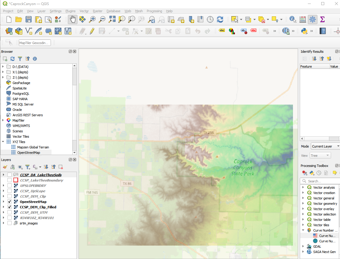
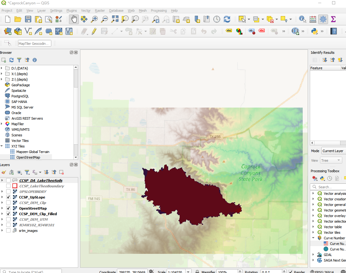
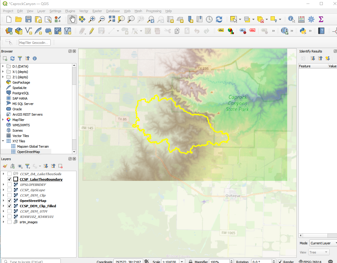
GIS Soils Properties#
From the discussion regarding infiltration, it should be apparent that soil properties are important. There
Paper-Based Maps#
Well just kidding, the old soils maps (of my generation) are archived at USDA Soil Surveys
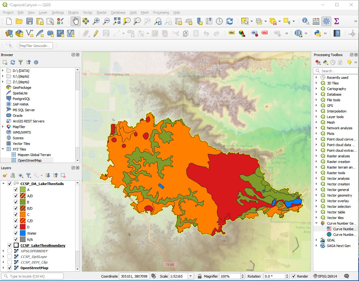
An example watershed at Caprock Canyon (called the Lake Theo watershed in my notes) is in Briscoe Co. Texas
Here is the soils map Briscoe Co. Tx Soils Maps (with text)
The study location is Map sheet 51 in the document.
The main mapped soils are QBG,BeB, and BeC. In the same document are tables that reference these codes back to soil descriptions.
From the tables we obtain various estimates as:
Soil |
\(K_{sat}\)(in/hr) |
\(\approx~n\) (from AWC value) |
\(\approx~D_{50}\) (from sieve data)(mm) |
|---|---|---|---|
QBG |
2.0-6.0 |
0.10-0.20 |
0.074 |
BeB |
0.6-2.0 |
0.14-0.17 |
0.42-0.074 |
BeC |
0.6-2.0 |
0.14-0.17 |
0.42-0.074 |
As you will see in the in-class demonstration; the process to find these values is a bit slow - one can imagine the difficulties over larger areas, however it does provide meaningful values to parameterize one of the various infiltration models. We still need some way to approximate soil suction (or mean pore size) we can certainly use a guess of \(D_{50}\) we can estimate from the soils map as a surogate for pore size to estimate a suction value.
Now we recall from our Fluids class something like:
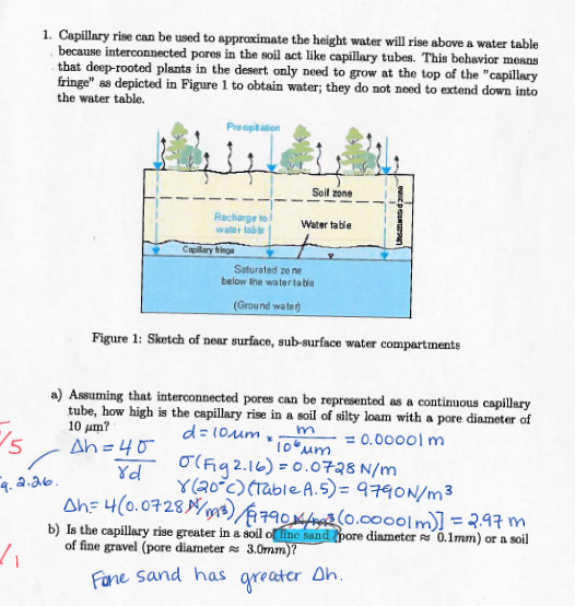
So with some guess of the \(D_{50}\) we can estimate the suction from a capillary rise approximation.
\(h_c = \frac{4 \sigma}{\gamma d}\)
surface_tension = 0.0728 # N/m
sp_weight = 9790 #N/cu.m.
diameter = 0.074e-3 #meters
capillary_rise = (4*surface_tension)/(sp_weight*diameter)
print("  Surface Tension ",round(surface_tension,3)," N/m")
print("  Specific Weight (of liquid) ",round(sp_weight,3)," N/cu.m.")
print("  Mean Pore Diameter ",round(1000*diameter,3)," mm\n ")
print("Capillary Rise ",round(capillary_rise,3)," m")
  Surface Tension  0.073  N/m
  Specific Weight (of liquid)  9790  N/cu.m.
  Mean Pore Diameter  0.074  mm

Capillary Rise  0.402  m
This capillary rise is a useful surrogate for the suction pressure in the infiltration models. For instance a Green-Ampt model for these soils would be something like:
\(I(t)=K_{sat}t + (H+h_c)ln(1+\frac{I(t)}{(H+h_c)n})\)
In our case \(h_c\approx 15~in.\); \(K_{sat} \approx 2.0~\frac{in.}{hr}\); and \(n \approx 0.20\) or something to this effect. So later on we can use this to estimate loss (and potential runoff).
GIS Data#
There is a soil survey geographic database at USDA Soils Data Gateway
You can also access from WSS in the navigation column USDA Web Soil Survey
An alternative is to use CN Generator Plug-In
3.2 Evapotranspiration Process and Factors Affecting It#
Evapotranspiration (ET) is a fundamental process in the hydrologic cycle, representing the combined loss of water from a watershed to the atmosphere through two pathways: evaporation from soil and water surfaces, and transpiration from plant leaves. Like infiltration, it is one of the key hydrologic abstractions that determines how much precipitation is ultimately available to generate runoff or recharge groundwater. In effect, evapotranspiration acts as a “leak” from the land-atmosphere interface, returning water to the sky before it ever appears in rivers or aquifers.
This process is especially important when modeling long-term water balances, irrigation needs, or climate impacts on watersheds. Even in regions with ample rainfall, high evapotranspiration rates can leave surprisingly little water for streamflow or groundwater recharge. ET is thus a critical consideration in both water supply planning and drought vulnerability assessments.
Evapotranspiration rates depend on a complex interplay of meteorological, biological, and physical factors, including temperature, solar radiation, humidity, wind speed, vegetation type, and soil moisture availability. For instance, well-watered crops on a hot, windy day can lose large volumes of water via transpiration. On the other hand, if soil moisture is depleted, ET becomes limited by water availability rather than energy inputs.
Roles in Hydrology:#
Water Budget Closure: ET is a major component in the closing of water balance equations for a watershed. It often accounts for a significant proportion of incoming precipitation—especially in arid and semi-arid regions.
Agricultural Planning: Understanding ET is vital for irrigation scheduling, crop selection, and yield forecasting. It dictates how much supplemental water may be needed to maintain healthy vegetation.
Climate Interactions: ET is also a feedback mechanism in climate models. It influences local humidity, cloud formation, and even precipitation patterns by regulating the amount of moisture returned to the atmosphere.
Factors Affecting Evapotranspiration:#
Vegetation Cover: Different plants have varying transpiration rates, with forested areas typically exhibiting higher ET than barren or urbanized lands.
Climatic Variables: Temperature, wind, solar radiation, and relative humidity all influence the potential evapotranspiration rate. Arid regions often have high potential ET even if actual ET is limited by water availability.
Soil Moisture: Availability of water in the root zone constrains how much can be transpired. When soil dries out, ET drops regardless of atmospheric demand.
Engineering and Management Strategies:#
Irrigation Efficiency: Using drip irrigation, soil moisture sensors, and crop-specific watering schedules can optimize water use and reduce unnecessary evapotranspiration losses.
Vegetative Planning: Selecting drought-tolerant or low-ET plant species in landscaping and agriculture can reduce overall water demand.
Remote Sensing and Modeling: Satellite-based tools and models like the Penman-Monteith equation help estimate ET over large areas, supporting regional water resource planning.
This schematic shows evapotranspiration as part of the watershed-scale water budget:
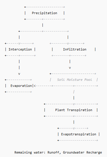
This flowchart illustrates the flux paths for precipitation as the water either evaporates, transpires, or continues to become runoff or groundwater recharge, depending on conditions.
TWDB Database#
3.3 Empirical Models for Estimating Evapotranspiration#
In many practical situations, direct measurements of evapotranspiration (ET) are unavailable. In such cases, empirical models are used to estimate ET based on climatological data. These models are particularly useful for agricultural planning, water resource assessments, and hydrologic modeling. Among the most widely used are the \textbf{Blaney-Criddle}, \textbf{Thornthwaite}, and \textbf{Turc} models. Each is relatively simple to implement in spreadsheet form and relies on limited climatic inputs.
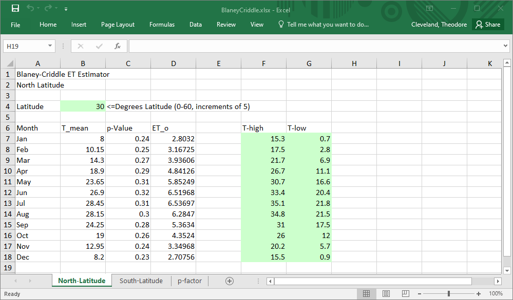
Blaney-Criddle Method#
The Blaney-Criddle model is a temperature- and latitude-based approach primarily used to estimate reference evapotranspiration \(ET_o\) for agricultural water use.
where
\(T\) = mean daily temperature for the month (°C)
\(p\) = mean daily percentage of annual daytime hours (dependent on latitude and month)
Key Characteristics
Simple and driven by temperature and latitude only.
Best suited for monthly time steps in warm-season climates.
Requires a crop coefficient (\(K_c\)) for estimating actual ET.
Limited accuracy in highly variable or humid climates due to lack of humidity, wind, or radiation input.
Use Case Quick estimates of ET when only temperature and location are known, especially in arid or semi-arid regions.
Spreadsheet Implementation The figure below is an example illustrating the simiplcity of the Blaney-Criddle estimation method. The figure is also a link to the spreadsheet.
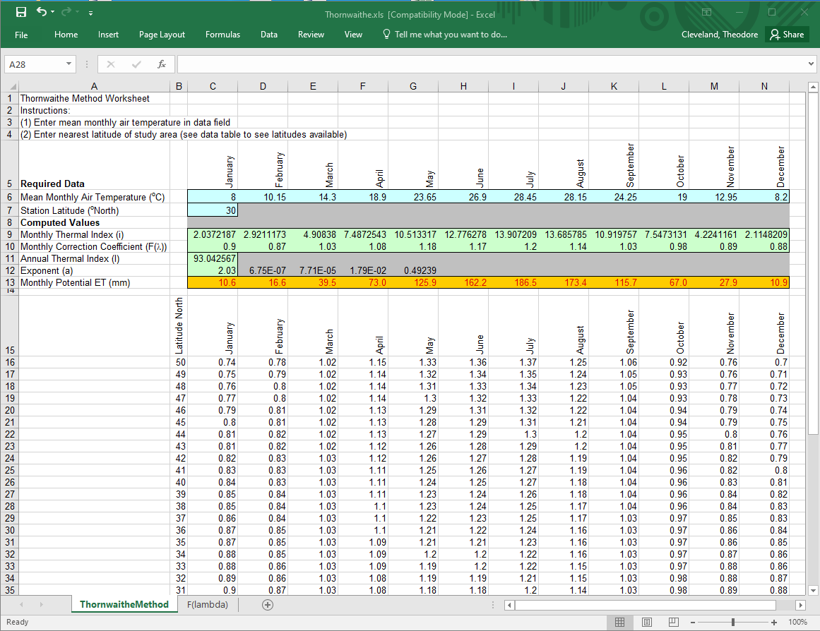
Thornthwaite Method#
The Thornthwaite model estimates potential evapotranspiration \(PET\) using monthly mean temperature and a calculated heat index.
where
\(T\) = mean monthly temperature (°C)
\(L\) = average day length (hours)
\(N\) = number of days in the month
\(I\) = annual heat index, computed as \(\sum \left( \frac{T}{5} \right)^{1.514}\)
\(a\) = empirical exponent derived from \(I\)
Key Characteristics
Incorporates photoperiod (day length) corrections.
Requires a full year of temperature data to compute the heat index and exponent.
Best suited for humid and temperate climates.
Overestimates ET in arid or tropical regions.
Use Case Suitable for long-term water balance modeling and ecological or climate classification studies.
Spreadsheet Implementation The figure below is an example illustrating the simiplcity of the Thornwaithe estimation method, the only required inputs are the latitude and mean monthly air temperatures. The figure is also a link to the spreadsheet.
Turc Model#
The Turc model is an empirical approach incorporating mean temperature and mean relative humidity, offering improved sensitivity to atmospheric moisture conditions.
A common simplified form:
Alternatively, with solar radiation:
where
\(T\) = average air temperature (°C)
\(U\) = mean relative humidity (%)
\(R\) = solar radiation (MJ/m\textsuperscript{2}/day), if available
Key Characteristics
More refined than Blaney-Criddle or Thornthwaite in humid climates.
Includes humidity sensitivity and optional radiation inputs.
Assumes well-watered conditions, estimating potential ET.
Use Case Effective in temperate and Mediterranean climates with reliable humidity or radiation data; appropriate for regional-scale hydrologic studies.
Spreadsheet Implementation
Warning
Need to find the Turc spreadsheet and copy to server -
Penman-Monteith Method#
The Penman-Monteith method is a physically based model that estimates reference evapotranspiration(ETo) by combining principles of energy balance and aerodynamic (mass transfer) theory. It is regarded as a robust method for ET estimation and is recommended by the Food and Agriculture Organization (FAO) as the standard formulation.
The method balances two key drivers:
Energy availability at the surface (via net radiation)
Atmospheric demand (via wind speed, temperature, and humidity gradients)
FAO Penman-Monteith Equation (standardized form)
Where:
\(ETo\) = reference evapotranspiration (mm/day)
\(R_n\) = net radiation at the crop surface (MJ/m\textsuperscript{2}/day)
\(G\) = soil heat flux density (MJ/m\textsuperscript{2}/day)
\(T\) = mean daily air temperature at 2 m height (°C)
\(u_2\) = wind speed at 2 m height (m/s)
\(e_s - e_a\) = saturation vapor pressure deficit (kPa)
\(\Delta\) = slope of vapor pressure curve (kPa/°C)
\(\gamma\) = psychrometric constant (kPa/°C)
Key Characteristics
Integrates both energy and aerodynamic terms—physically grounded.
Requires a range of meteorological inputs: temperature, radiation, humidity, and wind speed.
Used as the benchmark for other methods; all crop coefficients (\(K_c\)) are based on this reference ET.
Flexible enough to be applied to daily, monthly, or hourly time steps.
Use Case Accurate estimation of ET for irrigation scheduling, climate impact studies, and hydrologic modeling where detailed climate data are available. Widely implemented in agricultural and water resource planning tools.
Example 1: Simple Monthly Water Budget#
A basic water balance can be used to estimate actual evapotranspiration (AET):
Precipitation, \(P = 100\) mm/month
Runoff, \(R = 25\) mm/month
Infiltration = 50 mm/month
Groundwater Recharge, \(G = 10\) mm/month
Assuming negligible interception and storage change, the water balance is:
Solving for evapotranspiration:
Example 2: Penman-Monteith Reference ET Estimate#
Using the FAO Penman-Monteith equation to estimate reference evapotranspiration (\(ETo\)) under summer conditions:
Net radiation, \(R_n = 8\) MJ/m\textsuperscript{2}/day
Air temperature, \(T = 25^\circ\)C
Wind speed at 2 m, \(u_2 = 2\) m/s
Saturation vapor pressure deficit, \(e_s - e_a = 2.0\) kPa
Psychrometric constant, \(\gamma = 0.066\) kPa/°C
Slope of vapor pressure curve, \(\Delta = 0.188\) kPa/°C
Substituting values:
Compute step-by-step:
This result represents the reference ET under well-watered grass conditions.
3.4 Data Science Approach#
The Data Science Approach to evapotranspiration estimation uses observed meteorological and hydrologic data to build statistical or machine learning models that approximate ET based on historical patterns. This method is particularly useful in regions where pan evaporation, temperature, and rainfall data are available, but complete energy balance or aerodynamic measurements are lacking.
Rather than relying on physical or semi-empirical equations, this approach leverages data-driven relationships between evapotranspiration and climate variables using regression models, time series techniques, or advanced machine learning algorithms.
Key Data Inputs (from available sources):
Precipitation (P)
Pan evaporation (E\textsubscript{pan}) and net evaporation (if available)
Temperature (T)
Solar radiation (R), if available
Month or seasonal indicator variables
An example form of a predictive model might be:
Where:
\(T_{3p}\) = 3-period moving average of temperature
\(P_{3p}\) = 3-period moving average of precipitation
\(R_{3p}\) = 3-period moving average of solar radiation
Key Characteristics
Flexible and adaptable to regional data availability
Can be calibrated using local observations (e.g., Texas pan evaporation datasets)
Allows incorporation of lagged variables, seasonal trends, and nonlinear responses
May outperform empirical models in regions with dense, high-quality observational networks
Use Case Ideal for operational forecasting, drought monitoring, or spatial mapping of ET where sufficient historical data exist. Particularly useful when computational resources permit model fitting and validation.
Data Source Example Texas Water Development Board’s evaporation and rainfall data portal https://waterdatafortexas.org/lake-evaporation-rainfall
Example 3. Evaporation Trend Examination (Data Science Approach)#
Global warming is a currently popular and hotly (pun intended) debated issue. The usual evidence is temperature data presented as a time series with various temporal correlations to industrial activity and so forth. The increase in the global temperature is not disputed - what it means for society and how to respond is widely disputed.
One possible consequence of warming, regardless of the cause is an expectation that evaportation rates would increase and temperate regions would experience more drought and famine, and firm water yields would drop.
However in a paper by Peterson and others (1995) the authors concluded from analysis of pan evaporation data in various parts of the world, that there has been a downward trend in evaporation at a significance level of 99%. Pan evaporation is driven as much by direct solar radiation (sun shining on water) as by surrounding air temperature.
Global dimming is defined as the decrease in the amounts of solar radiation reaching the surface of the Earth. The by-product of fossil fuels is tiny particles or pollutants which absorb solar energy and reflect back sunlight into space. This phenomenon was first recognized in the year 1950. Scientists believe that since 1950, the sun’s energy reaching Earth has dropped by 9% in Antarctica, 10% in the USA, 16% in parts of Europe and 30% in Russia – putting the overall average drop to be at an enormous 22%. This causes a high risk to our environment.
Aerosols have been found to be the major cause of global dimming. The burning of fossil fuels by industry and internal combustion engines emits by-products such as sulfur dioxide, soot, and ash. These together form particulate pollution—primarily called aerosols. Aerosols act as a precursor to global dimming in the following two ways:
These particle matters enter the atmosphere and directly absorb solar energy and reflect radiation back into space before it reaches the planet’s surface. Water droplets containing these air-borne particles form polluted clouds. These polluted clouds have a heavier and larger number of droplets. These changed properties of the cloud – such clouds are called ‘brown clouds’ – makes them more reflective. Vapors emitted from the planes flying high in the sky called contrails are another cause of heat reflection and related global dimming.
Both global dimming and global warming have been happening all over the world and together they have caused severe changes in the rainfall patterns. It is also believed that it was global dimming behind the 1984 Saharan drought that killed millions of people in sub-Saharan Africa. Scientists believe that despite the cooling effect created by global dimming, the earth’s temperature has increased by more than 1 deg. in the last century.
References#
Example Problem#
In Texas, evaporation rates (reported as inches per month) are available from the Texas Water Development Board. https://waterdatafortexas.org/lake-evaporation-rainfall The map below shows the quadrants (grid cells) for which data are tabulated.
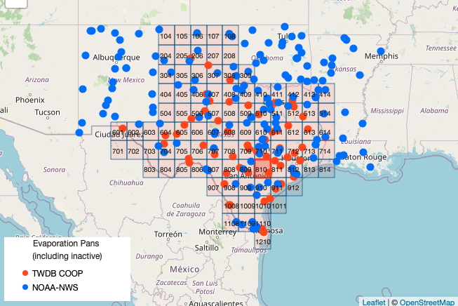
Cell ‘911’ is located between Corpus Christi and Houston in the Coastal Plains of Texas. A copy of the dataset downloaded from the Texas Water Development Board is located at http://www.rtfmps.com/share_files/all_quads_gross_evaporation.csv
Using naive data science anlayze the data for Cell ‘911’ and decide if the conclusions by Peterson and others (1995) are supported by this data.
Exploratory Analysis#
To analyze these data a first step is to obtain the data. The knowlwdge that the data are arranged in a file with a .csv extension is a clue how to proceede. We will need a module to interface with the remote server, in this example lets use something different than urllib. Here we will use requests , so first we load the module
import requests # Module to process http/https requests
import pandas as pd
Now we will generate a GET request to the remote http server. I chose to do so using a variable to store the remote URL so I can reuse code in future projects. The GET request (an http/https method) is generated with the requests method get and assigned to an object named rget – the name is arbitrary. Next we extract the file from the rget object and write it to a local file with the name of the remote file - esentially automating the download process. Then we import the pandas module.
remote_url="http://54.243.252.9/ce-3354-webroot/hydrohandbook/chapters/03-infiltration/all_quads_gross_evaporation.csv"  # set the url
rget = requests.get(remote_url, allow_redirects=True)  # get the remote resource, follow imbedded links
open('all_quads_gross_evaporation.csv','wb').write(rget.content) # extract from the remote the contents, assign to a local file same name
import pandas as pd # Module to process dataframes (not absolutely needed but somewhat easier than using primatives, and gives graphing tools)
Now we can read the file contents and check its structure, before proceeding.
evapdf = pd.read_csv("all_quads_gross_evaporation.csv",parse_dates=["YYYY-MM"]) # Read the file as a .CSV assign to a dataframe evapdf
evapdf.head() # check structure
| YYYY-MM | 104 | 105 | 106 | 107 | 108 | 204 | 205 | 206 | 207 | ... | 911 | 912 | 1008 | 1009 | 1010 | 1011 | 1108 | 1109 | 1110 | 1210 | |
|---|---|---|---|---|---|---|---|---|---|---|---|---|---|---|---|---|---|---|---|---|---|
| 0 | 1954-01-01 | 1.80 | 1.80 | 2.02 | 2.24 | 2.24 | 2.34 | 1.89 | 1.80 | 1.99 | ... | 1.42 | 1.30 | 2.50 | 2.42 | 1.94 | 1.29 | 2.59 | 2.49 | 2.22 | 2.27 |
| 1 | 1954-02-01 | 4.27 | 4.27 | 4.13 | 3.98 | 3.90 | 4.18 | 4.26 | 4.27 | 4.26 | ... | 2.59 | 2.51 | 4.71 | 4.30 | 3.84 | 2.50 | 5.07 | 4.62 | 4.05 | 4.18 |
| 2 | 1954-03-01 | 4.98 | 4.98 | 4.62 | 4.25 | 4.20 | 5.01 | 4.98 | 4.98 | 4.68 | ... | 3.21 | 3.21 | 6.21 | 6.06 | 5.02 | 3.21 | 6.32 | 6.20 | 5.68 | 5.70 |
| 3 | 1954-04-01 | 6.09 | 5.94 | 5.94 | 6.07 | 5.27 | 6.31 | 5.98 | 5.89 | 5.72 | ... | 3.83 | 3.54 | 6.45 | 6.25 | 4.92 | 3.54 | 6.59 | 6.44 | 5.88 | 5.95 |
| 4 | 1954-05-01 | 5.41 | 5.09 | 5.14 | 4.40 | 3.61 | 5.57 | 4.56 | 4.47 | 4.18 | ... | 3.48 | 3.97 | 7.92 | 8.13 | 6.31 | 3.99 | 7.75 | 7.98 | 7.40 | 7.40 |
5 rows × 93 columns
Structure looks like a spreadsheet as expected; lets plot the time series for cell ‘911’
evapdf.plot.line(x='YYYY-MM',y='506') # Plot quadrant 911 evaporation time series
<Axes: xlabel='YYYY-MM'>
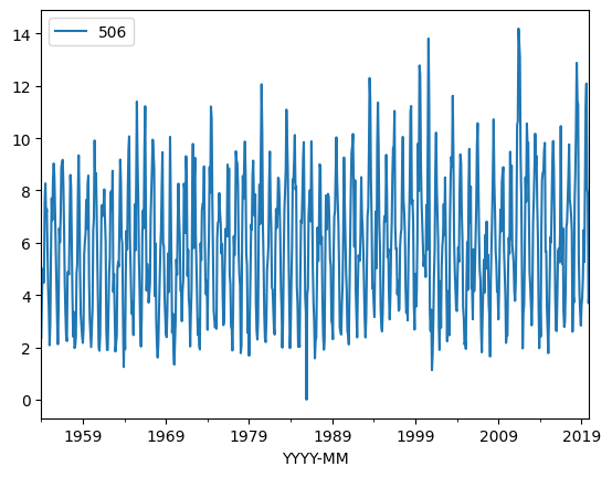
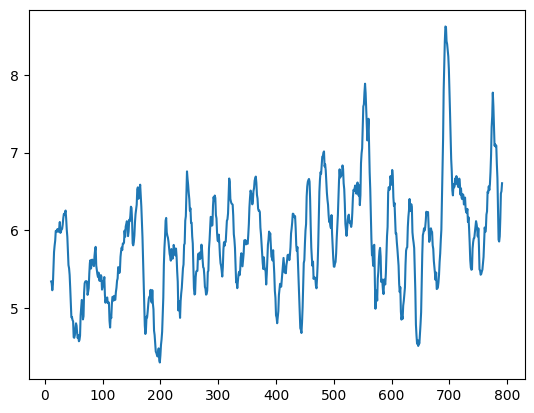
Now we can see that the signal indeed looks like it is going up at its mean value then back down. Lets try a moving average over 12-month windows. The syntax is a bit weird, but it should dampen the high frequency (monthly) part of the signal. Sure enough there is a downaward trend at about month 375, which we recover the date using the index – in this case around 1985.
movingAvg=evapdf['506'].rolling(12, win_type ='boxcar').mean()
movingAvg
movingAvg.plot.line(x='YYYY-MM',y='506')
evapdf['YYYY-MM'][375]
evapdf['506'].describe()
count    792.000000
mean       5.858346
std        2.562598
min        0.000000
25%        3.710000
50%        5.750000
75%        7.740000
max       14.190000
Name: 506, dtype: float64
So now lets split the dataframe at April 1985. Here we will build two objects and can compare them. Notice how we have split into two entire dataframes.
evB485loc = evapdf['YYYY-MM']<'1985-04'  # filter before 1985
evB485 = evapdf[evB485loc]
ev85uploc = evapdf['YYYY-MM']>='1985-04' # filter after 1985
ev85up= evapdf[ev85uploc]
print(evB485.head())
print(ev85up.head())
     YYYY-MM   104   105   106   107   108   204   205   206   207  ...   911  \
0 1954-01-01  1.80  1.80  2.02  2.24  2.24  2.34  1.89  1.80  1.99  ...  1.42
1 1954-02-01  4.27  4.27  4.13  3.98  3.90  4.18  4.26  4.27  4.26  ...  2.59
2 1954-03-01  4.98  4.98  4.62  4.25  4.20  5.01  4.98  4.98  4.68  ...  3.21
3 1954-04-01  6.09  5.94  5.94  6.07  5.27  6.31  5.98  5.89  5.72  ...  3.83
4 1954-05-01  5.41  5.09  5.14  4.40  3.61  5.57  4.56  4.47  4.18  ...  3.48

    912  1008  1009  1010  1011  1108  1109  1110  1210
0  1.30  2.50  2.42  1.94  1.29  2.59  2.49  2.22  2.27
1  2.51  4.71  4.30  3.84  2.50  5.07  4.62  4.05  4.18
2  3.21  6.21  6.06  5.02  3.21  6.32  6.20  5.68  5.70
3  3.54  6.45  6.25  4.92  3.54  6.59  6.44  5.88  5.95
4  3.97  7.92  8.13  6.31  3.99  7.75  7.98  7.40  7.40

[5 rows x 93 columns]
       YYYY-MM   104    105    106   107   108   204    205    206   207  ...  \
375 1985-04-01  5.31   6.27   6.75  6.92  4.76  5.32   6.72   6.83  7.04  ...
376 1985-05-01  4.80   5.64   5.51  5.47  5.43  4.90   6.62   6.37  6.13  ...
377 1985-06-01  6.61   9.00   9.05  8.66  8.33  6.39   8.62   8.33  7.55  ...
378 1985-07-01  7.21  10.99  11.10  9.73  8.56  7.30  10.11  10.33  9.40  ...
379 1985-08-01  6.56   9.66   9.76  8.48  7.38  6.31   8.85   8.55  7.45  ...

      911   912  1008  1009  1010  1011  1108  1109  1110  1210
375  4.16  4.45  5.26  5.06  4.91  4.41  6.24  5.58  4.81  4.63
376  5.87  5.17  5.19  5.66  5.69  5.86  5.63  5.59  5.63  5.71
377  6.60  6.46  5.91  5.98  6.03  6.41  6.33  6.17  6.38  6.12
378  7.56  6.64  6.50  7.18  7.09  7.41  7.10  7.18  7.13  7.27
379  8.37  6.93  7.76  8.44  8.72  8.52  8.09  7.94  8.35  8.57

[5 rows x 93 columns]
Now lets get some simple descriptions of the two objects, and we will ignore thay they are time series.
evB485['911'].describe()
count    375.000000
mean       4.202480
std        1.774273
min        1.260000
25%        2.665000
50%        3.900000
75%        5.455000
max        8.800000
Name: 911, dtype: float64
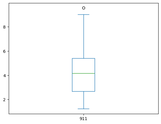
ev85up['911'].describe()
count    417.000000
mean       4.167458
std        1.676704
min        1.230000
25%        2.680000
50%        4.160000
75%        5.410000
max        9.560000
Name: 911, dtype: float64
If we look at the means, the after 1985 is lower, and the SD about the same, so there is maybe support of the paper claims, but the median has increased while the IQR is practically unchanged. We can produce boxplots from the two objects and see they are different, but not by much. So the conclusion of the paper has support but its pretty weak and hardly statisticlly significant.
evB485['911'].plot.box()
<Axes: >
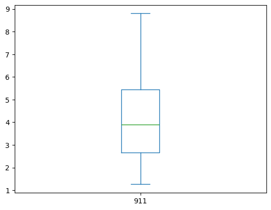
ev85up['911'].plot.box()
<Axes: >
At this point, we would appeal to hypothesis testing or some other serious statistical analysis tools. Lets try a favorite (of mine) non-paramatric test called the mannwhitneyu test.
Background#
In statistics, the Mann–Whitney U test (also called the Mann–Whitney–Wilcoxon (MWW), Wilcoxon rank-sum test, or Wilcoxon–Mann–Whitney test) is a nonparametric test of the null hypothesis that it is equally likely that a randomly selected value from one population will be less than or greater than a randomly selected value from a second population.
This test can be used to investigate whether two independent samples were selected from populations having the same distribution.
Application#
As usual we need to import necessary tools, in this case scipy.stats. Based on the module name, it looks like a collection of methods (the dot . is the giveaway). The test itself is applied to the two objects, if there is a statistical change in behavior we expect the two collections of records to be different.
from scipy.stats import mannwhitneyu # import a useful non-parametric test
stat, p = mannwhitneyu(evB485['911'],ev85up['911'])
print('statistic=%.3f, p-value at rejection =%.3f' % (stat, p))
if p > 0.05:
	print('Probably the same distribution')
else:
	print('Probably different distributions')
statistic=78190.500, p-value at rejection =0.999
Probably the same distribution
If there were indeed a 99% significance level, the p-value should have been smaller than 0.05 (two-tailed) and the p-value was quite high. I usually check that I wrote the script by testing he same distribution against itself, I should get a p-vale of 0.5. Indeed that’s the case.
stat, p = mannwhitneyu(evB485['911'],evB485['911'])
print('statistic=%.3f, p-value at rejection =%.3f' % (stat, p))
if p > 0.05:
	print('Probably the same distribution')
else:
	print('Probably different distributions')
statistic=70312.500, p-value at rejection =1.000
Probably the same distribution
Now lets repeat the analysis but break in 1992 when Clean Air Act rules were slightly relaxed:
evB492loc = evapdf['YYYY-MM']<'1992'  # filter before 1992
evB492 = evapdf[evB492loc]
ev92uploc = evapdf['YYYY-MM']>='1992' # filter after 1992
ev92up= evapdf[ev92uploc]
#print(evB492.head())
#print(ev92up.head())
stat, p = mannwhitneyu(evB492['911'],ev92up['911'])
print('statistic=%.3f, p-value at rejection =%.3f' % (stat, p))
if p > 0.05:
	print('Probably the same distribution')
else:
	print('Probably different distributions')
statistic=81021.000, p-value at rejection =0.166
Probably the same distribution
So even considering the key date of 1992, there is marginal evidence for the claims (for a single spot in Texas), and one could argue that the claims are confounding – as an FYI this evevtually was a controversial paper because other researchers obtained similar results using subsets (by location) of the evaporation data.
Explore More#
Using data science tools anlayze the data for Cell ‘911’ and decide if the conclusions by Peterson and others (1995) are supported by this data. That is, do the supplied data have a significant trend over time in any kind of grouping?
Some things you may wish to consider as you design and implement your analysis are: Which summary statistics are relevant?
Ignoring the periodic signal, are the data approximately normal? Are the data homoscedastic? What is the trend of the entire dataset (all years)? What is the trend of sequential decades (group data into decades)? What is the trend of sequential 15 year groups? Is there evidence that the slope of any of the trends is zero? At what level of significance?
Some additional things to keep in mind:
1. These data are time series; serial correlation is present.
2. An annual-scale periodic signal is present
We have not yet discussed time series analysis and periodic signals. Peterson and others (1995) only analyzed May through September data, does using this subset of data change your conclusions?
Exercise(s)#
ce3354-es2-2025-3.pdf ET and Infiltration Exercises