6. Streamflow Measurement and Streamflow Data#
Course Website
Readings#
Chow, V.T., Maidment, D.R., Mays, L.W., 1988, Applied Hydrology: New York, McGraw-Hill. pp. 1-12
See 7-31 TxDOT HDM for a description of slope-area (slope-conveyance) method
Generalized Skew Update and Regional Study of Distribution Shape for Texas Flood Frequency Analyses
Jamie Chan (2014) Learn Python in One Day and Learn It Well. LCF Publishing. Kindle Edition.
Grus, Joel. Data Science from Scratch: First Principles with Python. O’Reilly Media. Kindle Edition.
https://www.amazon.com/Distributional-Statistics-Environment-Statistical-Computing/dp/1463508417
https://www.astroml.org/book_figures/chapter3/fig_gamma_distribution.html
https://www.inferentialthinking.com/chapters/10/Sampling_and_Empirical_Distributions.html
https://www.inferentialthinking.com/chapters/15/Prediction.html
Videos#
How to look at and download streamflow data from the USGS NWIS website
Precipitation Runoff Modeling System (PRMS) Streamflow Modules
Improved process based streamflow simulation through ensemble and stochastic data driven approaches
Hydrology - Statistical Hydrology 2 (go to time stamp 47:00 to get to regionalization)
Streamflow Measurement(s)#
Streamflow tells us how much water is flowing past a certain point in a stream or river. Streamflow (or discharge) affects almost all aspects of stream health, including essential biological and chemical processes. Many institutions, agencies, organizations, and landowners rely on an accurate accounting of streamflow for the estimation of pollutant and nutrient loading, prediction of flood levels, and other environmental management activities.
The United States Geological Survey (USGS) defines streamflow as “the volumetric rate of flow of water (volume per unit time) in an open channel, including any sediment or other solids that may be dissolved or mixed with it that adhere to the Newtonian physics of open-channel hydraulics of water.” Discharge is in open channel flow or the passage of water through flumes, culverts, and other non-pressurized conveyances. Generally, discharge Q (ft3/s or m3/s) is calculated as the product of a mean section velocity v (ft/s or m/s) of water moving through a unit area A (ft2 or m2):
Q = v * A
Magnitudes of discharge range widely depending on the size and location of the stream as well as groundwater levels and recent precipitation. For example, the average discharge in the Mississippi River at Baton Rouge, Louisiana, ranges between 308,000 and 843,000 ft3/s (or cfs). Average discharge in the Saluda River near Greenville, South Carolina, ranges between 347 and 1040 cfs, and discharge in small, shallow streams in South Carolina is often below a single (1.0) cfs.2
Stream gaging is either:
Continuous record (usually stage, then rated to produce discharge)
Located at control section if possible
Crest-Stage (captures peak stage)
Uses slope-area to estimate discharge
Post-event site visit required to survey debris-line as independent check of estimate
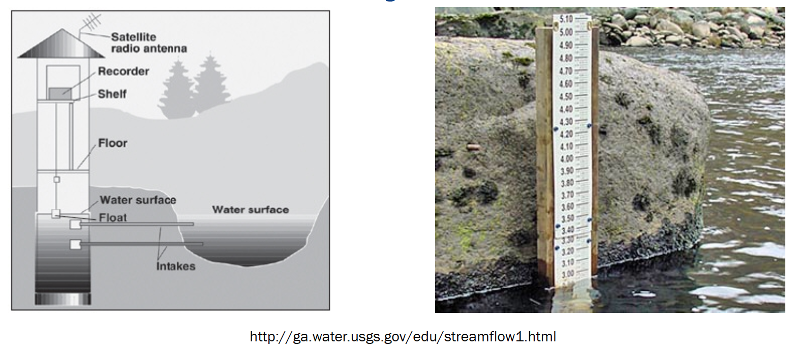
Stream stage is often referenced when discussing river conditions and the quantity of water within a river. Stream stage refers to how high the water surface is above a pre-defined elevation point in the stream which is often the streambed or even an absolute elevation. Rises and falls in the stream stage (also referred to as stage or gage height) indicate changes in streamflow. This relationship between stream stage and discharge is referred to as the stage-discharge relationship. Stream stage can be measured using sensors such as pressure transducers, water level radar, bubblers, and cameras, or stage can be measured using staff gauges, crest-stage gauges, or measure-downs from a defined point. Stream stage is then related to a series of stream discharge measurements across a wide range of streamflow conditions to create a stage-discharge relationship or rating curve. This rating curve can then be used to estimate flow during most flow conditions within a range of flow measurements, assuming consistent boundary conditions. Rating curves should be updated as vegetation, erosion, and sedimentation affect discharge in the stream section, which vary in some streams to a near-constant state of change to an almost completely steady state.1,4
Measurement Techniques#
Streamflow is measured by a variety of gaging technologies. Measuring Streamflow
Weirs
Flumes
Velocity-area methods
Continuous gages use some kind of stilling well, and transducers to measure stage and send to satellite. During visits, a nearby staff gage is read to independently validate the transducer readings
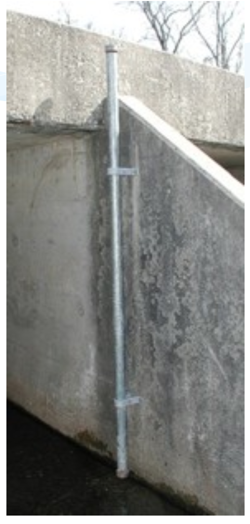
Crest-Stage gagues usually consist of a vertical pipe with holes in bottom – becomes a stilling well. Inside a staff gage and small amount of cork “flour” records water surface elevation.
A hydrographer visits site routinely (and after major events) and records cork elevation and re-sets gage.
The elevations are marked on a staff inside the pipe with pencil (and dated)
Slope area method between several nearby pipes is used to estimate discharge
Slope Area Method#
Application of Manning’s equation, using the slope of the water surface as the friction slope, and the stage geometry at measured cross sections.
Recall the factor 1.49 is for US Customary units, 1.0 is used if terms are expressed in SI units.
Acoustic Doppler Current Profiler (ADCP)#
An Acoustic Doppler Current Profiler, or Acoustic Doppler Profiler, is often referred to with the acronym ADCP.
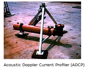
Scientists use the instrument to measure how fast water is moving across an entire water column. An ADCP (uplooking) anchored to the seafloor can measure current speed not just at the bottom, but also at equal intervals all the way up to the surface.
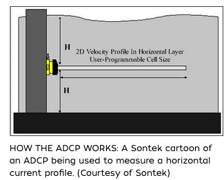
The instrument can also be mounted horizontally on seawalls or bridge pilings in rivers and canals to measure the current profile from shore to shore, and to the bottoms of ships to take constant current measurements as the boats move. In very deep areas, they can be lowered on a cable from the surface.
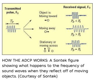
The ADCP measures water currents with sound, using a principle of sound waves called the Doppler effect. A sound wave has a higher frequency, or pitch, when it moves to you than when it moves away. You hear the Doppler effect in action when a car speeds past with a characteristic building of sound that fades when the car passes.
The ADCP works by transmitting “pings” of sound at a constant frequency into the water. (The pings are so highly pitched that humans and even dolphins can’t hear them.) As the sound waves travel, they ricochet off particles suspended in the moving water, and reflect back to the instrument. Due to the Doppler effect, sound waves bounced back from a particle moving away from the profiler have a slightly lowered frequency when they return. Particles moving toward the instrument send back higher frequency waves. The difference in frequency between the waves the profiler sends out and the waves it receives is called the Doppler shift. The instrument uses this shift to calculate how fast the particle and the water around it are moving.
Sound waves that hit particles far from the profiler take longer to come back than waves that strike close by. By measuring the time it takes for the waves to bounce back and the Doppler shift, the profiler can measure current speed at many different depths with each series of pings.
Note
Acoustic Doppler Current Profilers (ADCPs) provide direct measurements of flow velocity across a cross-section, in contrast to traditional stage-based methods, where water surface elevation (stage) is recorded continuously and discharge is inferred using a pre-established stage–discharge rating curve. Both approaches are widely used in streamflow monitoring. While stage data remain essential—at minimum—to define cross-sectional geometry and support rating curve development, continuous velocity profiling is less commonly implemented due to cost and deployment complexity. However, advances in sensor technology and data telemetry are rapidly increasing the feasibility of high-frequency, velocity-based discharge monitoring at both permanent and temporary sites.
Streamflow Data#
Data sources for streamflow include both national and international networks:
USGS NWIS (USA) – National Water Information System (https://waterdata.usgs.gov/)
IBWC – International Boundary and Water Commission (US–Mexico border data)
Older “paper-based” records – Agency archives, academic institutions, engineering reports
Local gage networks – Operated by water authorities, municipalities, or research entities
WMO Global Runoff Data Centre (GRDC) – Hosted by BfG Germany, offering global river discharge data (https://www.bafg.de/GRDC)
European Water Archive (EWA) – Historic river flow data from European countries (via GRDC collaboration)
Australian Bureau of Meteorology Water Data – Streamflow and hydrology data portal (http://www.bom.gov.au/waterdata/)
HydroSHEDS and HydroRIVERS – Global hydrographic datasets suitable for modeling and estimation (https://www.hydrosheds.org/)
FAO AQUASTAT – Global water statistics including streamflow where available (http://www.fao.org/aquastat/)
National Hydrological Services – Most countries operate a national hydrology or water resources agency that publishes data
Note
When using international data, it’s essential to check metadata for temporal resolution, measurement standards, and quality control protocols, as these may differ from U.S.-based sources.
Illustrative workflow using USGS NWIS#
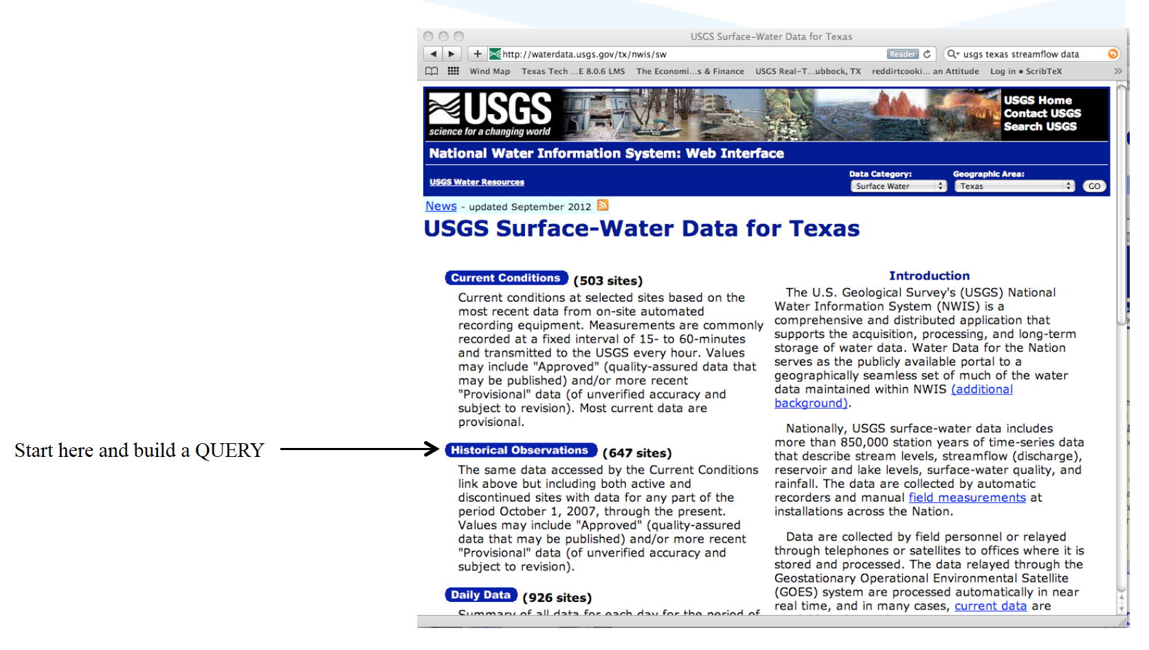
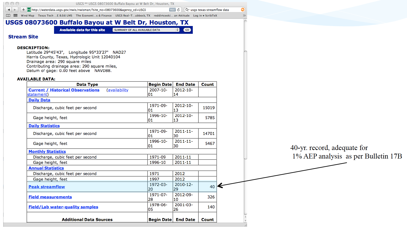
The U.S. Geological Survey’s National Water Information System (NWIS) is the primary source for streamflow data in the United States. The following workflow demonstrates how to retrieve historical discharge data from NWIS using a web-based interface.
Begin by navigating to the NWIS landing page for the state or territory of interest. This can be accessed via the main USGS Water Data site or by searching for “NWIS [State Name]”. The state page provides an overview of all monitored sites and offers a search tool to help filter by county, basin, site type, or parameter.
Once on the state-specific NWIS page, use the interactive map or filtering tools to locate a stream gage station at or near your study area. For most hydrologic analyses, proximity and physiographic similarity are important, so selecting a station “stupid close” (i.e., geographically and hydrologically relevant) is preferable. The example shown highlights a site near Houston, Texas, which is suitable for demonstration purposes.
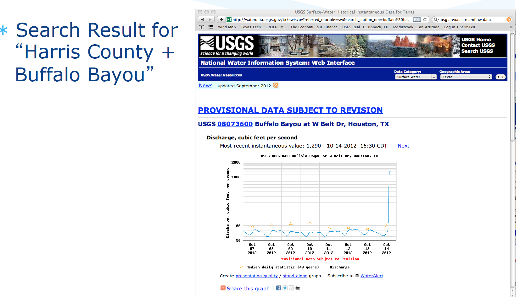
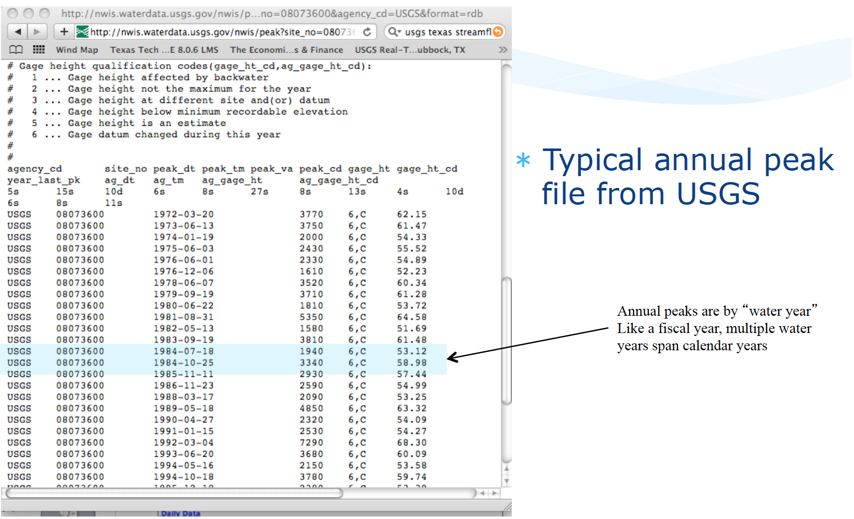
Clicking on the station name brings up its dedicated site summary page, which includes metadata such as gage location, drainage area, period of record, and available parameters. Scroll to the “Available data for this site” section and choose the discharge (streamflow) dataset, usually expressed in cubic feet per second (cfs). You can specify a date range and choose the output format—commonly tab-delimited RDB format or comma-separated CSV—and then download the file to your local system.
The resulting file includes a structured header with metadata followed by time series values. For example, a daily mean streamflow record will list the date, mean flow, and a flag column indicating data qualifiers (e.g., estimated values). This structure makes it relatively easy to import into Excel, Python, or statistical software for further analysis.
Tip
When working with NWIS data, always inspect the header rows carefully—they often contain important notes about data quality, revisions, and units.
Hydrograph Analysis and Baseflow Separation#
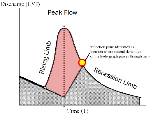
A hydrograph is a time series plot that shows how streamflow or discharge varies over time at a particular point in a watershed, typically following a rainfall event. It reflects the integrated response of a watershed to precipitation, modulated by surface and subsurface flow processes.
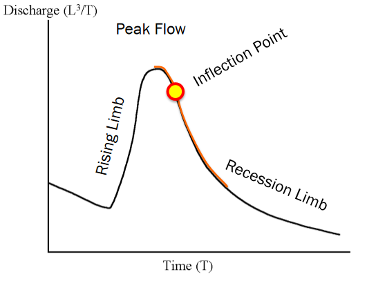
The idealized hydrograph is divided into:
Rising limb: where discharge increases rapidly due to incoming runoff
Peak flow: the highest point of the hydrograph, representing the maximum discharge
Recession limb: the gradual decrease in flow as runoff and baseflow subside
In engineering hydrology, peak flow estimation is essential for:
Designing culverts, bridges, detention ponds
Urban drainage systems
Flood risk assessments
In engineering hydrology, entire hydrograph estimation is important for
Modeling the temporal distribution of runoff for detention and retention system design
Assessing watershed response for hydrologic and hydraulic simulation models
Supporting water quality analysis and long-term water resource planning
The hydrograph pictured also has a baseflow component – Flow in the absence of a storm, often contributed by groundwater discharge or delayed interflow. – During storm events, total streamflow consists of both baseflow and stormflow (direct runoff) components. – To estimate peak flow or the entire storm hydrograph, it is important to separate the baseflow from the observed hydrograph. – This separation is essential for understanding rainfall-runoff relationships and for use in modeling, design, and watershed assessments.
To perform baseflow separation, several graphical methods have been developed. Common approaches include:
Constant discharge method#
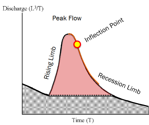
Identify the point where the rising limb begins.
Assign that flow value as a constant baseflow rate throughout the storm event.
Connect this baseflow rate across the event duration until it re-joins the recession limb.
The portion of flow above the constant line is considered stormflow.
Constant slope method#
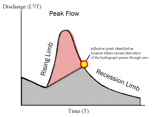
Identify the point where the rising limb begins.
Draw a straight line from this point to the inflection point on the recession limb.
The area above this line is treated as stormflow.
Limitations: Difficult to apply accurately in hydrographs with multiple peaks.
Concave method#
Begin at the rising limb, and trace a concave curve downward along the recession limb, ending beneath the hydrograph peak.
Then draw a second segment from this point to the inflection point on the falling limb.
The region above these segments is defined as stormflow.
Limitations: Can be subjective, especially when dealing with multi-peaked hydrographs.
Other Techniques#
The Master Depletion Curve Method, described in course readings, is useful for long-term or event-specific hydrograph separation using established depletion patterns.
For complex or continuous simulations, automated baseflow separation techniques or hydrologic modeling tools (e.g., SWAT, HEC-HMS) may be more appropriate.
In practice, the constant discharge method is often favored for multi-peaked events due to its simplicity and reproducibility.