Logistic Regression
Background
Multiple Variable Models
\begin{gather} \mathbf{\beta}= \begin{pmatrix} \beta_0 \ \beta_1 \ \vdots \ \beta_m \ \end{pmatrix} \end{gather} $$
The matrix has as many rows as observations to fit, and as many columns as predictor variables.
Fitting Process
The logistic regression method attempts to find values of \(\beta\) that minimizes the log-likelihood function
The presence of the last term makes the process a search process (instead of a single equation to solve), some form of iterative least squares. In general we will rely on packages to handle this work - an example follows
Read the database
import pandas as pd
import numpy as np
import sklearn.metrics as metrics
import matplotlib.pyplot as plt
import seaborn as sns
%matplotlib inline

mydatabase = pd.read_csv('LogisticRegressionHomebrewExample.csv')
Verify the read, and plot the database
mydatabase.describe()
| X1 | X2 | Class | |
|---|---|---|---|
| count | 20000.000000 | 20000.000000 | 20000.000000 |
| mean | 0.496920 | 2.001764 | 0.500000 |
| std | 1.113666 | 2.240266 | 0.500013 |
| min | -4.214002 | -3.489115 | 0.000000 |
| 25% | -0.260873 | -0.015846 | 0.000000 |
| 50% | 0.498444 | 1.978725 | 0.500000 |
| 75% | 1.264066 | 4.016432 | 1.000000 |
| max | 4.605613 | 7.945987 | 1.000000 |
#Split dataframe based on class value and plot
classone = mydatabase[mydatabase['Class']<1.0]
classzero = mydatabase[mydatabase['Class']>0.0]
# plot the two classes as red and blue
plt.figure(figsize=(10, 8))
plt.scatter(classzero['X1'],classzero['X2'], c="red", alpha=0.3)
plt.scatter(classone['X1'],classone['X2'], c="blue", alpha=0.3)
plt.legend(["Class 0","Class 1"])
plt.xlabel('X1 Predictor')
plt.ylabel('X2 Predictor')
plt.grid(which='both')
plt.show()

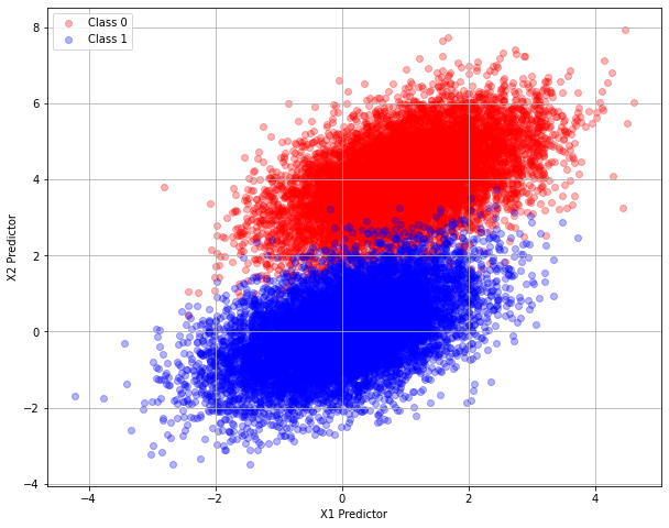
The two classes appear different enough so the logistic-regression classification seems possible. For example if the predictor input is \([0,0]\) then the class is likely “Class 1”, whereas if the predictor input is \([0,4]\) then the class is likely “Class 0” according to the above plot.
#split dataset in features and target variable
feature_cols = ['X1', 'X2']
X = mydatabase[feature_cols] # Features
y = mydatabase["Class"] # Target variable
# split X and y into training and testing sets
from sklearn.model_selection import train_test_split
X_train,X_test,y_train,y_test=train_test_split(X,y,test_size=0.25,random_state=0)
# import the class
from sklearn.linear_model import LogisticRegression

# instantiate the model (using the default parameters)
#logreg = LogisticRegression()
logreg = LogisticRegression()
# fit the model with data
logreg.fit(X_train,y_train)

#
y_pred=logreg.predict(X_test)
# import the metrics class
from sklearn import metrics
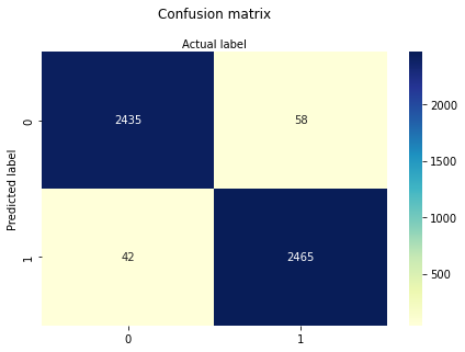
cnf_matrix = metrics.confusion_matrix(y_pred, y_test)
cnf_matrix
array([[2435,   58],
       [  42, 2465]])
class_names=[0,1] # name  of classes
fig, ax = plt.subplots()
tick_marks = np.arange(len(class_names))
plt.xticks(tick_marks, class_names)
plt.yticks(tick_marks, class_names)
# create heatmap
sns.heatmap(pd.DataFrame(cnf_matrix), annot=True, cmap="YlGnBu" ,fmt='g')
ax.xaxis.set_label_position("top")
plt.tight_layout()
plt.title('Confusion matrix', y=1.1)
plt.ylabel('Predicted label')
plt.xlabel('Actual label');

Now lets build a classification (class prediction) engine using logistic regression results.
First we need the sigmoid response function where
def sigmoid(scores): # scores = b0+b1X1+b2X2+... where b0,b1,b2,... are specified
    return 1/(1+np.exp(-scores))
Now lets use our two obvious values from the discussion above
inputs = np.array([[0],[1]]) # one example input, should evaluate as
scores = np.dot(logreg.coef_,inputs) + logreg.intercept_
estimated_class = sigmoid(np.dot(logreg.coef_,inputs) + logreg.intercept_)[0,0] # grab the only element
print("X1 Input = ",inputs[0][0],"\nX2 Input = ",inputs[1][0],"\nEstimated Class Value",round(estimated_class,0))
X1 Input =  0
X2 Input =  1
Estimated Class Value 0.0
inputs = np.array([[0],[4]]) # one example input, should evaluate as
scores = np.dot(logreg.coef_,inputs) + logreg.intercept_
estimated_class = sigmoid(np.dot(logreg.coef_,inputs) + logreg.intercept_)[0,0] # grab the only element
print("X1 Input = ",inputs[0][0],"\nX2 Input = ",inputs[1][0],"\nEstimated Class Value",round(estimated_class,0))
X1 Input =  0
X2 Input =  4
Estimated Class Value 1.0
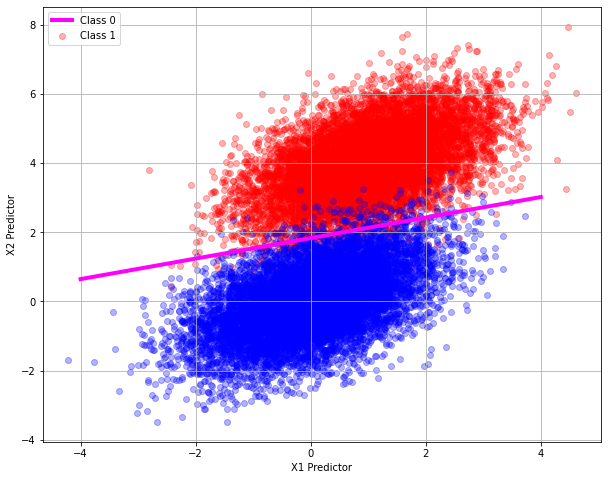
So now we have a classifer function, we could probably draw a dividing line back on the original plot and identify the dividing line, we only need two points where the classifier returns a value of 0.5 as below
inputs = np.array([[-4],[0.645]]) # one example input, should evaluate as
scores = np.dot(logreg.coef_,inputs) + logreg.intercept_
estimated_class = sigmoid(np.dot(logreg.coef_,inputs) + logreg.intercept_)[0,0] # grab the only element
print("X1 Input = ",inputs[0][0],"\nX2 Input = ",inputs[1][0],"\nEstimated Class Value",round(estimated_class,3))
X1 Input =  -4.0
X2 Input =  0.645
Estimated Class Value 0.502
inputs = np.array([[4],[3.018]]) # one example input, should evaluate as
scores = np.dot(logreg.coef_,inputs) + logreg.intercept_
estimated_class = sigmoid(np.dot(logreg.coef_,inputs) + logreg.intercept_)[0,0] # grab the only element
print("X1 Input = ",inputs[0][0],"\nX2 Input = ",inputs[1][0],"\nEstimated Class Value",round(estimated_class,3))
X1 Input =  4.0
X2 Input =  3.018
Estimated Class Value 0.5
Our two points by trial and error are: \([-4.0,0.645]\) and \([4.0,3.018]\) we can add this line to our plot
# plot the two classes as red and blue
plt.figure(figsize=(10, 8))
plt.scatter(classzero['X1'],classzero['X2'], c="red", alpha=0.3)
plt.scatter(classone['X1'],classone['X2'], c="blue", alpha=0.3)
plt.plot([-4,4],[0.645,3.018],c="magenta",linewidth=4)
plt.legend(["Class 0","Class 1"])
plt.xlabel('X1 Predictor')
plt.ylabel('X2 Predictor')
plt.grid(which='both')
plt.show()

Single Variable Models
A single variable model is a special case of the multi-variate approach with the following modifications:
A simple example follows:
toxicity = pd.DataFrame([[1,2,3,4,5,6],[28,53,93,126,172,197]],["Log_Dose","Deaths"] )
toxicity = toxicity.transpose()
toxicity.head()
# compute death fraction, all doses exposed to 250 subjects
toxicity["Fraction"]=toxicity["Deaths"]/250.0
# declare lethal id fraction >0.5

def islethal(value):
    if value >= 0.5:
        islethal = 1
    else:
        islethal = 0
    return(islethal)

toxicity["Class"]=toxicity["Fraction"].apply(islethal)
toxicity.head()
| Log_Dose | Deaths | Fraction | Class | |
|---|---|---|---|---|
| 0 | 1 | 28 | 0.112 | 0 |
| 1 | 2 | 53 | 0.212 | 0 |
| 2 | 3 | 93 | 0.372 | 0 |
| 3 | 4 | 126 | 0.504 | 1 |
| 4 | 5 | 172 | 0.688 | 1 |
def log_likelihood(features, target, weights): # features are the design variables; weights are the b0,b1,b2,...;target is the known class (0 or 1)
    scores = np.dot(features, weights)
    ll = np.sum(target * scores - np.log(1 + np.exp(scores)))
    return ll
def logistic_regression(features, target, num_steps, learning_rate, add_intercept=False, verbose=True, exit_tolerance = 1.0e-9):
    if add_intercept:
        intercept = np.ones((features.shape[0], 1))
        features = np.hstack((intercept, features))
# print statements are for debugging
    weights = np.zeros(features.shape[1])  # not sure about this line
    print("initial weights = ",weights)
    print("initial log likelihood = ",log_likelihood(features, target, weights))

#
    for step in range(num_steps):
        llold = log_likelihood(features, target, weights)
        if verbose: print("start weights = ",weights)
        scores = np.dot(features, weights)
        if verbose: print("start scores = ",scores)
        predictions = sigmoid(scores)
        if verbose: print("predictions = ",predictions)
        output_error_signal = target - predictions
        gradient = np.dot(features.T, output_error_signal)
        weights = weights + learning_rate * gradient
        if verbose: print("new weights = ",weights)
        newscores = np.dot(features, weights)
        if verbose: print("new scores = ",newscores)
        llnew = log_likelihood(features, target, weights)

# test for exit
        if abs(llnew-llold) <= exit_tolerance:
            print("Exit Tolerance Satisfied \n  LL is not changing")
            print("step = ",step)
            print("ll = ",log_likelihood(features, target, weights))
            break # exit the loop
        if step % 5 == 0:
            if verbose: print("step = ",step)
            if verbose: print("ll = ",log_likelihood(features, target, weights))
            if verbose: print("error signal = ",output_error_signal)
            if verbose: print("predictions = ",predictions)
# print on exit
    print("step = ",step)
    print("ll = ",log_likelihood(features, target, weights))
    print("error signal = ",output_error_signal)
    print("predictions = ",predictions)
    return weights
Produce a design matrix using numpy and the dataframe we read. Similarily the class vector (of 0’s and 1’s) is constructed from the dataframe. These new objects have row-wise correspondence; that is a row of designmatrix corresponds to the same row of classvector. In terms of the above expressions
$\(\text{classvector} = Y_{obs} \)$
$\(\text{designmatrix} = X\)$
designmatrix = mydatabase[["X1","X2"]].to_numpy()
classvector = mydatabase["Class"].to_numpy()
These are supplied to our regression machine
betas = logistic_regression(designmatrix, classvector, 900, 0.00001, add_intercept=False, verbose=False)
initial weights =  [0. 0.]
initial log likelihood =  -13862.943611198905
Exit Tolerance Satisfied
  LL is not changing
step =  621
ll =  -8139.368262867247
step =  621
ll =  -8139.368262867247
error signal =  [-0.4258073  -0.69253714 -0.32390763 ...  0.04174041  0.01879931
  0.0332575 ]
predictions =  [0.4258073  0.69253714 0.32390763 ... 0.95825959 0.98120069 0.9667425 ]
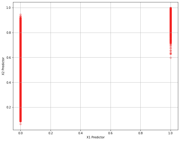
modelvector = sigmoid(np.dot(designmatrix, betas))
# plot the two classes as red and blue
plt.figure(figsize=(10, 8))
plt.scatter(classvector,modelvector, c="red", alpha=0.3)
#plt.scatter(classone['X1'],classone['X2'], c="blue", alpha=0.3)
#plt.legend(["Class 0","Class 1"])
plt.xlabel('X1 Predictor')
plt.ylabel('X2 Predictor')
plt.grid(which='both')
plt.show()

modelvector[1]
0.6925371237744782
classvector[100]
0
sigmoid(np.dot([0,2], betas))
0.8509476740456239
sigmoid(np.dot([0,4], betas))
0.9702321502038639
