Applications - Electronic Circuit Analysis
Solving a Circuit (using Linear Algebra)
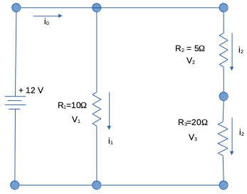
Suppose we wish to analyze the electric circuit in Fig. 2.

Fig. 12 Caption
In this example, identical to the earlier example, we will employ a few tricks to generalize the solution for nearly any resistor network in a DC circuit. The actual result is a modification of an algorithm presented by Haman and Braemiller (CITE). Applying the problem solving protocol might be something like
Step 1: Problem Statement
Determine the unknown parameters that characterize the behavior of the circuit depicted in Fig. 2.
Step 2: Sketch the Situation
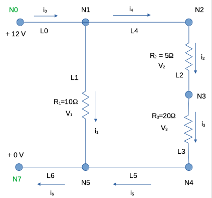
To employ the linear-system approach of Haman and Braemiller (CITE) we will need to redraw the sketch a bit as

Fig. 13 Caption
Step 3: List Known and Unknown Values
Known:
Circuit topology (configuration) and component relative locations.
Source voltage: +12 volts as shown on the diagram.
Resistor values: \(R_1=~10 \Omega\) , \(R_2=~5 \Omega\) , \(R_3=~20 \Omega\)
Unknown:
The current in different parts of the circuit: \(i_0\) , \(i_1\) , \(i_2\) .
The voltage drops (differences) across each resistor: \(V_1\) , \(V_2\) , \(V_3\) .
Step 4: Identify Governing Principles
Ohm’s law: The voltage drop across a resistor is the product of current frowing through the resistor and the resistance; \(V=IR\) .
Kirchoff’s Law - Resistors in Series; \(R_T=R_1 + R_2 + \dots+ R_n\)
Kirchoff’s Law - Resistors in Parallel; \(R_T=\frac{1}{\frac{1}{R_1} + \frac{1}{R_2} + \dots+ \frac{1}{R_n}}\)
We don’t actually need Kirchoff’s Law in the method we will employ, mostly just Ohm’s law and continunity of current at a node. We will solve for voltages at each node, and currents in each link.
Step 5: Analysis
Different from the last time we examined this problem, we will simply write continunity of charge at each node:
\(\sum i_{inflow} - \sum i_{outflow} = 0\) at each node (note if we have capicators and/or inductors, then there is a storage term and the system is no longer at equilibrium). So we will end up with one equation for each interior node (Node 0 and Node 7 have known voltages).
For example for Node 1:
\(i_0 - i_1 - i_4 = 0\) is the current balance equation for the node.
Next we will implement Ohm’s law for each link; for example for Link 1:
\(V_1 - R_1 i_1 -V_5 = 0\)
Next simply organize these into a system of equations and solve. For this example the equation system looks like:
Where the link resistances are set to a small, but non-zero value to preserve the non-singularity of the coefficient matrix, except for links with known resistances, and the known node voltages appear in the RHS vector.
Step 6 Implementing a solver in the Jupyter Notebook
First we will prototype in Jupyter Lab and explicitly enter the matrix coefficients and right-hand-side. Once we recognize the node-arc pattern, we can modify our script to operate on just a minimal description supplied by an external datafile.
import numpy
nnodes = 5
nlinks = 6
R0 = 0.00001 # small but non-zero to prevent singular matrix
R1 = 10.0
R2 =  5.0
R3 = 20.0
R4 = 0.00001 # small but non-zero to prevent singular matrix
R5 = 0.00001 # small but non-zero to prevent singular matrix
R6 = 0.00001 # small but non-zero to prevent singular matrix
#           [i0, i1, i2, i3, i4, i5, i6, v1, v2, v3, v4, v5]
amatrix = [[  1, -1,  0,  0, -1,  0,  0,  0,  0,  0,  0,  0],
           [  0,  0, -1,  0,  1,  0,  0,  0,  0,  0,  0,  0],
           [  0,  0,  1, -1,  0,  0,  0,  0,  0,  0,  0,  0],
           [  0,  0,  0,  1,  0, -1,  0,  0,  0,  0,  0,  0],
           [  0,  1,  0,  0,  0,  1, -1,  0,  0,  0,  0,  0],
           [-R0,  0,  0,  0,  0,  0,  0, -1,  0,  0,  0,  0],
           [  0,-R1,  0,  0,  0,  0,  0,  1,  0,  0,  0, -1],
           [  0,  0,-R2,  0,  0,  0,  0,  0,  1, -1,  0,  0],
           [  0,  0,  0,-R3,  0,  0,  0,  0,  0,  1, -1,  0],
           [  0,  0,  0,  0,-R4,  0,  0,  1, -1,  0,  0,  0],
           [  0,  0,  0,  0,  0,-R5,  0,  0,  0,  0,  1, -1],
           [  0,  0,  0,  0,  0,  0,-R6,  0,  0,  0,  0,  1]]
rhsvector = [0,0,0,0,0,-12,0,0,0,0,0,0]
# use numpy for the linear algebra
A = numpy.array(amatrix)# numpy the A matrix
b = numpy.array(rhsvector)# numpy the b vector
x = numpy.linalg.solve(A,b) # solve the linear system, x marks the spot
# debug
#for i in range(len(amatrix)):
#    print(amatrix[i],rhsvector[i],round(x[i],3))
print("--------Node Voltages--------")
for i in range(1,nnodes+1,1):
    print("Voltage at Node",i," is ",round(x[nlinks+i],3)," Volts")
print("--------Link Currents--------")
for i in range(0,nlinks+1,1):
    print("Current in Link ",i," is ",round(x[i],3)," Amperes")
--------Node Voltages--------
Voltage at Node 1  is  12.0  Volts
Voltage at Node 2  is  12.0  Volts
Voltage at Node 3  is  9.6  Volts
Voltage at Node 4  is  0.0  Volts
Voltage at Node 5  is  0.0  Volts
--------Link Currents--------
Current in Link  0  is  1.68  Amperes
Current in Link  1  is  1.2  Amperes
Current in Link  2  is  0.48  Amperes
Current in Link  3  is  0.48  Amperes
Current in Link  4  is  0.48  Amperes
Current in Link  5  is  0.48  Amperes
Current in Link  6  is  1.68  Amperes
