Fitting a Line to Data Using Packages
So in core python, there is a fair amount of work involved to write a script to fit data - how about an easier way?
Using packages specifically designed for line fitting is that easier way!
Using statsmodel
First lets get things into a dataframe. Using the lists from the example above we can build a dataframe using pandas.
Note
Here we are cheating a little because we already know what packages we want to use
#Load the necessary packages
import numpy as np
import pandas as pd
import statistics
from matplotlib import pyplot as plt
import statsmodels.formula.api as smf # here is the regression package to fit lines
Now build a dataframe
distance = [2,4,11,7,17]
force = [2.0,3.5,8.0,4.5,9.5]
data = pd.DataFrame({'X':distance, 'Y':force}) # we use X,Y as column names for simplicity
data.head()
| X | Y | |
|---|---|---|
| 0 | 2 | 2.0 |
| 1 | 4 | 3.5 |
| 2 | 11 | 8.0 |
| 3 | 7 | 4.5 |
| 4 | 17 | 9.5 |
Now we will define and fit a linear model to the data, observe the rather simple syntax, no for-loops!
# Initialise and fit linear regression model using `statsmodels`
model = smf.ols('Y ~ X', data=data) # model object constructor syntax
model = model.fit()
Now to get output from the model, first we will generate a summary table
print(model.summary())
                            OLS Regression Results
==============================================================================
Dep. Variable:                      Y   R-squared:                       0.958
Model:                            OLS   Adj. R-squared:                  0.944
Method:                 Least Squares   F-statistic:                     68.00
Date:                Wed, 20 Jul 2022   Prob (F-statistic):            0.00373
Time:                        16:43:55   Log-Likelihood:                -4.3518
No. Observations:                   5   AIC:                             12.70
Df Residuals:                       3   BIC:                             11.92
Df Model:                           1
Covariance Type:            nonrobust
==============================================================================
                 coef    std err          t      P>|t|      [0.025      0.975]
------------------------------------------------------------------------------
Intercept      1.2794      0.611      2.094      0.127      -0.665       3.224
X              0.5147      0.062      8.246      0.004       0.316       0.713
==============================================================================
Omnibus:                          nan   Durbin-Watson:                   1.872
Prob(Omnibus):                    nan   Jarque-Bera (JB):                0.884
Skew:                           0.993   Prob(JB):                        0.643
Kurtosis:                       2.453   Cond. No.                         18.1
==============================================================================

Notes:
[1] Standard Errors assume that the covariance matrix of the errors is correctly specified.
/opt/jupyterhub/lib/python3.8/site-packages/statsmodels/stats/stattools.py:74: ValueWarning: omni_normtest is not valid with less than 8 observations; 5 samples were given.
  warn("omni_normtest is not valid with less than 8 observations; %i "
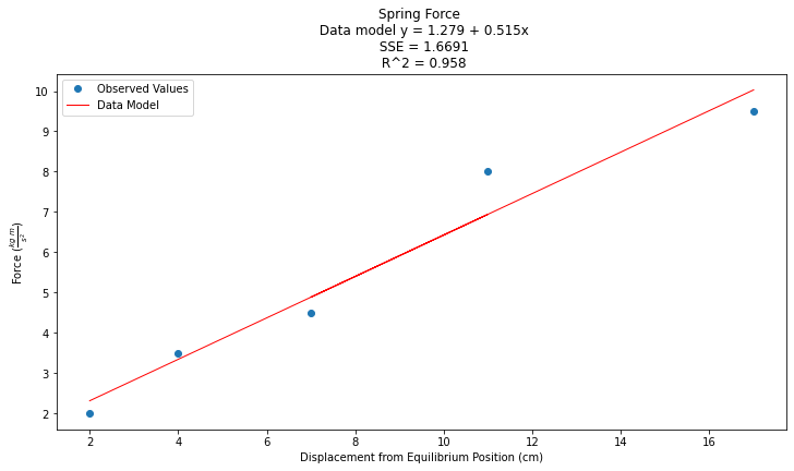
The model parameters are contained in a tuple named model.params which we could query for making a plot. Below we will access this as well as some other values from the fitting tool. We can get a listing of all the available properties from the package documentation
# Predict values
y_pred = model.predict()

beta0 = model.params[0] # the fitted intercept
beta1 = model.params[1]
sse = model.ssr
rsq = model.rsquared

titleline = "Spring Force \n Data model y = " + str(round(beta0,3)) + " + " + str(round(beta1,3)) + "x" # put the model into the title
titleline = titleline + '\n SSE = ' + str(round(sse,4)) + '\n R^2 = ' + str(round(rsq,3))

# Plot regression against actual data
plt.figure(figsize=(12, 6))
plt.plot(data['X'], data['Y'], 'o')           # scatter plot showing actual data
plt.plot(data['X'], y_pred, 'r', linewidth=1)   # regression line
plt.xlabel('Displacement from Equilibrium Position (cm)')
plt.ylabel('Force '+r'($\frac{kg~m}{s^2}$)')
plt.legend(['Observed Values','Data Model'])
plt.title(titleline)

plt.show();

Using sklearn
Again we will use dataframes from pandas. We have some reading to do at the sklearn documentation site.
# repeat using sklearn
# Multiple Linear Regression with scikit-learn:
from sklearn.linear_model import LinearRegression

# Build linear regression model using X as predictors
# Split data into predictors X and output Y
predictors = ['X'] # this seems odd, but will make sense when we add predictors later
X = data[predictors]
y = data['Y']

# Initialise and fit model
lm = LinearRegression()  # This is the sklearn model tool here
model = lm.fit(X, y)
Now the model is fit next we
Make predictions (
sklearnspecific calls)Recover the betas
Compute SSE and \(R^2\)
Build a plot
# Predict values
y_pred = model.predict(X)

beta0 = model.intercept_ # the fitted intercept
beta1 = model.coef_[0]

from sklearn.metrics import mean_squared_error, r2_score
sse = len(y)*mean_squared_error(y,y_pred) # shenigians here to get value same as homebrew
rsq = r2_score(y,y_pred) # no shenigians here, but goofy ass function call


titleline = "Spring Force \n Data model y = " + str(round(beta0,3)) + " + " + str(round(beta1,3)) + "x" # put the model into the title
titleline = titleline + '\n SSE = ' + str(round(sse,4)) + '\n R^2 = ' + str(round(rsq,3))

# Plot regression against actual data
plt.figure(figsize=(12, 6))
plt.plot(data['X'], data['Y'], 'o')           # scatter plot showing actual data
plt.plot(data['X'], y_pred, 'r', linewidth=1)   # regression line
plt.xlabel('Displacement from Equilibrium Position (cm)')
plt.ylabel('Force '+r'($\frac{kg~m}{s^2}$)')
plt.legend(['Observed Values','Data Model'])
plt.title(titleline)

plt.show();

At this point we certainly have tools to fit straight lines.
Summary
Use of a package greatly simplifies curve fitting, but we have to read how to use a package.
The goal is to fit a data model to data
statsmodelprovides a nice interface, obtain same results as our homebrew scriptssklearnis another package, also same resultsUse the package you like, plot your results to check your conclusions
Warning
The plots become tricky using the packages. Here they look fine, but are actually flawed because the plot series are not sorted. Remember line plots expect sorted x-values. When we get to later plots we amy have to sort the predictions to get the plots to look decent.
