.ipynb .pdf

repository open issue

Binder

Contents

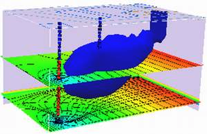
2D Plume in Regional Flow with 1st-Order Decay (Wilson and Miller Solution)

The sketch depicts a vertical line source in an aquifer of infinite extent located at (x,y)=(0,0) some time after constant injection has begun.

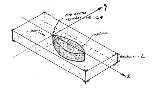
For the line source (injection well) whose fluid contribution makes negligible impact on the local hydraulics as depicted in the sketch the initial, boundary, and mass conservation conditions are:

\[C(x,y,0)=0\]

\[C(\pm \infty,\pm \infty,t)=0\]

\[\int_{- \infty}^{\infty}\int_{-\infty}^{\infty}C(x,y,t)dxdy = C_0 Q t\]

A solution obtained by time-convolution of an elementary line source solution with 1st order decay term is (Wilson and Miller, 1978) is

\[C(x,y,t) = \frac{C_0 Q}{4 \pi n L}\frac{1}{\sqrt{D_x D_y}}exp(\frac{x v}{2 D_x})W(u,\frac{r}{B})\]

where \(W(u,\frac{r}{B})\) is the leaky aquifer (Hantush) well function with

\[B=\frac{2D_x}{v}\]

\[d=1+\frac{2B\lambda}{v}\]

\[r= {\sqrt{(x^2+y^2\frac{D_x}{D_y})d}}\]

\[u=\frac{r^2}{4 d D_x t}\]

The solution is presented in (Bear and Cheng, 2010) as

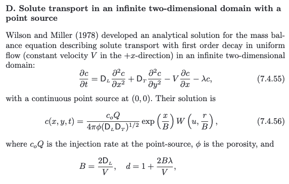
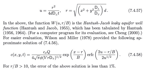a convolution integral (eqn. 10.6.38, p. 634) (the end user needs to supply the integration routine); Hunt (1978) noticed that the integral was the leaky well function with appropriate substitutions and completed the solution.

The leaky aquifer function can be evaluated numerically using a recursive definition, or efficient approximations can be used. Listings for these approximations appear below after the references

The solution is applicable for porous media flow, where the velocity (below) is the mean section velocity (seepage velocity divided by the porosity). The solution can also be used with streams and pipes (porosity = 1). Negative values of distance in x-axis would correspond to locations upgradient of the injection location.

Scripts to generate solutions are listed below:

Leaky Well Function

def wh(u, rho): # Hantush Leaky aquifer well function
    import numpy
    """Returns Hantush's well function values

    Note: works only for scalar values of u and rho

    Parameters:
    -----------
    u : scalar  (u= r^2 * S / (4 * kD * t))
    rho : sclaar (rho =r / lambda, lambda = sqrt(kD * c))
    Returns:
    --------
    Wh(u, rho) : Hantush well function value for (u, rho)
    """
    try:
        u =float(u)
        rho =float(rho)
    except:
        print("u and rho must be scalars.")
        raise ValueError()

    LOGINF = 2
    y = numpy.logspace(numpy.log10(u), LOGINF, 1000)
    ym = 0.5 * (y[:-1]+  y[1:])
    dy = numpy.diff(y)
    wh = numpy.sum(numpy.exp(-ym - (rho / 2)**2 / ym ) * dy / ym)
    return(wh)

Wilson and Miller Solution (Prototype Function)

def willsonmiller(c_injection,q_injection,l_thickness,d_x,d_y,decay,velocity,x_location,y_location,time):
    import math
    B   = 2*d_x/velocity
    d   = 1+2*B*decay/velocity
    rsq = (x_location**2 + (y_location**2)*(d_x/d_y))*d
    r   = math.sqrt(rsq)
    u   = rsq/(4.0*d*d_x*time)
#    print(B,d,rsq,r,u,r/B)
#    print(rsq,rrr,aaa,bbb)
    term1 = c_injection*q_injection/(4.0*math.pi*l_thickness)
    term2 = 1.0/(math.sqrt(d_x*d_y))
    term3 = math.exp((x_location*velocity)/(2.0*d_x))
    term4 = wh(u,r/B)

    #if term4 <= 0.0: term4 = 0.0
#    print(term1,term2,term3,term4)
    if term1*term2*term3*term4 <=0.0:
        temp = 0.0
    else:
        temp = term1*term2*term3*term4
    willsonmiller = temp
    return willsonmiller

Driver Script

# inputs
decay = 0#0.0024 # added 1st order decay
c_injection = 133
q_injection = 3.66
l_thickness = 1.75
d_x = 0.920
d_y = 0.092
velocity = 0.187
x_location = 123
y_location = 0
time = 36500
scale = c_injection*q_injection
output = willsonmiller(c_injection,q_injection,l_thickness,d_x,d_y,decay,velocity,x_location,y_location,time)
print("Concentration at x = ",round(x_location,2)," y= ",round(y_location,2) ," t= ",round(time,2) ," = ",repr(output))
#
print(wh(0.1,61.5))

Concentration at x =  123  y=  0  t=  36500  =  53.424298876849655
6.232529667098016e-28

#
# forward define and initialize vectors for a profile plot
#
how_many_points = 29   
deltat = 12.3
t = [0.0 for i in range(how_many_points)]  # constructor notation
c = [0.0 for i in range(how_many_points)]  # constructor notation

t[0]=1e-5 #cannot have zero time, so use really small value first position in list
#
# build the profile predictions
#
for i in range(0,how_many_points,1):
    if i > 0:
        t[i]=t[i-1]+deltat
    c[i] = willsonmiller(c_injection,q_injection,l_thickness,d_x,d_y,decay,velocity,x_location,y_location,t[i])

#
# Import graphics routines for picture making
#
from matplotlib import pyplot as plt
#
# Build and Render the Plot
#
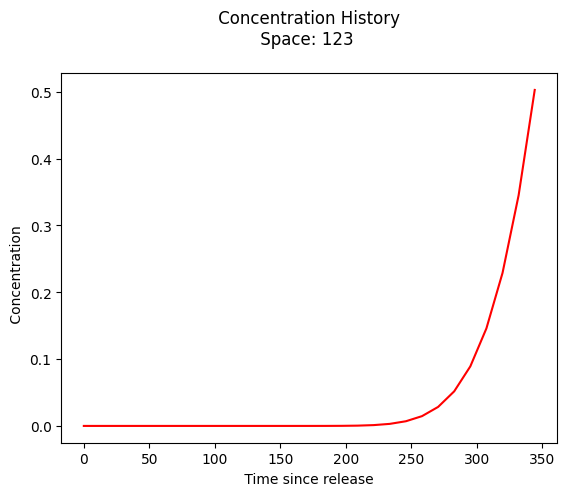
plt.plot(t,c, color='red', linestyle = 'solid')  # make the plot object
plt.title(" Concentration History \n Space: " + repr(x_location) + "  \n") # caption the plot object
plt.xlabel(" Time since release ") # label x-axis
plt.ylabel(" Concentration        ") # label y-axis
#plt.savefig("ogatabanksplot.png") # optional generates just a plot for embedding into a report
plt.show() # plot to stdio -- has to be last call as it kills prior objects
plt.close('all') # needed when plt.show call not invoked, optional here
#sys.exit() # used to elegant exit for CGI-BIN use

Plotting Script

# make a plot
x_max = 200
y_max = 100
# build a grid
nrows = 50   
deltax = (x_max*4)/nrows
x = []
x.append(-x_max)
for i in range(nrows):
    if x[i] == 0.0:
        x[i] = 0.00001
    x.append(x[i]+deltax)

ncols = 50   
deltay = (y_max*2)/(ncols-1)
y = []
y.append(-y_max)
for i in range(1,ncols):
    if y[i-1] == 0.0:
        y[i-1] = 0.00001
    y.append(y[i-1]+deltay)
    
#y

#y = [i*deltay for i in range(how_many_points)] # constructor notation
#y[0]=0.001
ccc = [[0 for i in range(nrows)] for j in range(ncols)]

for jcol in range(ncols):
    for irow in range(nrows):
        ccc[irow][jcol] = willsonmiller(c_injection,q_injection,l_thickness,d_x,d_y,decay,velocity,x[irow],y[jcol],time)
        
#y

my_xyz = [] # empty list
count=0
for irow in range(nrows):
    for jcol in range(ncols):
        my_xyz.append([ x[irow],y[jcol],ccc[irow][jcol] ])
       # print(count)
        count=count+1
        
#print(len(my_xyz))

import pandas
my_xyz = pandas.DataFrame(my_xyz) # convert into a data frame
import numpy 
import matplotlib.pyplot
from scipy.interpolate import griddata
# extract lists from the dataframe
coord_x = my_xyz[0].values.tolist() # column 0 of dataframe
coord_y = my_xyz[1].values.tolist() # column 1 of dataframe
coord_z = my_xyz[2].values.tolist() # column 2 of dataframe
#print(min(coord_x), max(coord_x)) # activate to examine the dataframe
#print(min(coord_y), max(coord_y))
coord_xy = numpy.column_stack((coord_x, coord_y))
# Set plotting range in original data units
lon = numpy.linspace(min(coord_x), max(coord_x), 64)
lat = numpy.linspace(min(coord_y), max(coord_y), 64)
X, Y = numpy.meshgrid(lon, lat)
# Grid the data; use linear interpolation (choices are nearest, linear, cubic)
Z = griddata(numpy.array(coord_xy), numpy.array(coord_z), (X, Y), method='cubic')
# Build the map
fig, ax = matplotlib.pyplot.subplots()
fig.set_size_inches(10, 5)
CS = ax.contour(X, Y, Z, levels = [1,5,10,15,20,25,30,35,40,45,50])
ax.clabel(CS, inline=2, fontsize=16)
ax.set_title('Concentration Map at Elapsed Time '+ str(round(time,1))+' days');

Spreadsheet Model

A spreadsheet implementation is available at http://54.243.252.9/ce-5364-webroot/6-Spreadsheets/WilsonMillerModel.xlsm

Note

This model requires Analysis Tool Pack Add-In and the VBA Macro Enabled.

References

1. Wilson, J.L. and Miller, P.J. (1978) Two-dimensional plumes in uniform groundwater flow. J. Hyd. Div., ASCE, 104:503–514, 1978.

2. Yuan, D, (1995) Accurate approximations for one-, two-, and three-dimensional groundwater mass transport from an exponentially decaying contaminant source. MS Thesis, Department of Civil and Environmental Engineering, University of Houston.

3. Chuang, Lu-Chia, (1998) A guidance system for choosing analytical contaminant transport models. Doctoral Dissertation, Department of Civil and Environmental Engineering, University of Houston, Houston, Texas. 222p.

4. Analytical solutions for one-, two-, and three-dimensional solute transport in ground-water systems with uniform flow Open-File Report 89-56

5. Analytical solutions for one-, two-, and three-dimensional solute transport in ground-water systems with uniform flow Techniques of Water-Resources Investigations 03-B7 (supercedes above reference)

previous

Analytical Models with Reaction Terms

next

Modeling Advection