4. Introduction to Modeling Environments#
Scope#
Overview of Jupyter Notebooks and Spreadsheets for analytical modeling
Introduction to MODFLOW6 and FLOPY (Groundwater Flow and Solute Transport)
Introduction to VS2DI (Variably Saturated Fluid Flow and Solute Transport)
Comparison of analytical and numerical approaches
Calculators and Spreadsheets#
These tools are useful for most of the 1D situations (with some programming 2D can be addressed using spreadsheets).
In most analytical solutions you will need some special functions:
erf() error function
erfc() complimentary error function
besseli(,) bessel function type i
besselj(,) bessel function type j
Ei() exponential integral
There are a few more, but these handle many of the cases. In Excel they are part of the Analysis Add-in, similarily with LibreOffice use Insert/Function/AddIn and a pull down menu appears with; alternatively they can be programmed using VBA and polynomial approximations to the functions.
Specialized Software#
More complex cases usually will require special software:
MODFLOW
MODPATH
MT3D
USGS-MOC (2D)
Chemflow-2000 are envisioned in this course.
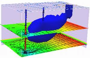
In many instances the output must be post processed to make graphical representations.
Note
We will probably use USGS-MOC, and output postprocessing for this course.
