2D - Advection-Dispersion, Finite-Width, Constant Source#
Note
This is one of several Domenico-based multi-dimension solutions. More will be added as time permits. Bear in mind that spatial convolution can be applied for constructing different source geometries, as can convolution (superposition in time) for different input histories.
The sketch depicts a finite-length horizontal line source in an aquifer of infinite extent located at \((x,y)=(0,0)\). The length of the source zone (line) is \(Y\).
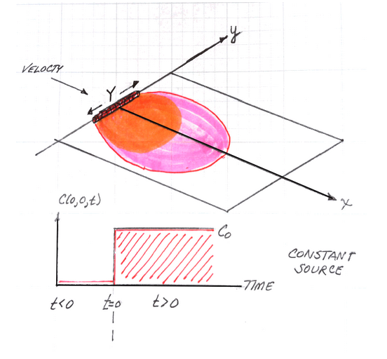
The source history is depicted beneath the sketch. The system starts with initial concentration of zero everywhere, at time \(t=0\), the concentration in the source line increases to \(C_0\) suddenly, and is maintained at that value from then on.
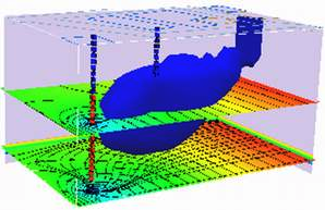
The transport processes modeled are advection along the x-axis, and dispersion in the x-direction (longitudinal) and in the y-direction (transverse).
The analytical model (Domenico and Robbins, 1985) was obtained by convolution of instantaneous sources (described in detail in Yuan, 1995):
A prototype function is
# prototype 2D domenico robbins ADE function
def c2ad(conc0, distx, disty, dispx, dispy, velocity, time, lenY):
    import math
    from scipy.special import erf, erfc # scipy needs to already be loaded into the kernel
    vadj = velocity / 1.0 # structure is in anticipation of adding adsorbtion and decay
    dispXadj = dispx / 1.0
    dispYadj = dispy / 1.0
    lambadj = 0 / 1.0

    uuu = math.sqrt(1.0 + 4.0*lambadj*dispXadj/vadj)
    ypp = (disty + 0.5*lenY) / (2*math.sqrt(dispYadj*distx))
    ymm = (disty - 0.5*lenY) / (2*math.sqrt(dispYadj*distx))

    arg1 = (distx - vadj*time*uuu) / (2*math.sqrt(dispXadj*vadj*time))
    arg2 = (distx / (2*dispXadj)) * (1 - uuu)

    term0 = conc0 / 4
    term1 = math.exp(arg2)
    term2 = erfc(arg1)
    term3 = (erf(ypp) - erf(ymm))

    c2ad = term0 * term1 * term2 * term3
    return c2ad
Supply model conditions, evaluate specific point in space and time.
# inputs
c_initial = 100.0 # g/m^3
xx = 100          # meters
yy = 0            # meters
Dx = 0.50          # m^2/day
Dy = 0.05          # m^2/day
V  = 1.0           # m/day
time = 100.0      # days
Y  = 10.0          # meters
alphax = Dx/V
alphay = Dy/V
output=c2ad(c_initial, xx, yy, alphax, alphay, V, time, Y)
print("x= ",round(xx,2)," y= ",round(yy,2)," t= ",round(time,1)," C(x,y,t) = ",round(output,3))
x= 100 y= 0 t= 100.0 C(x,y,t) = 44.308
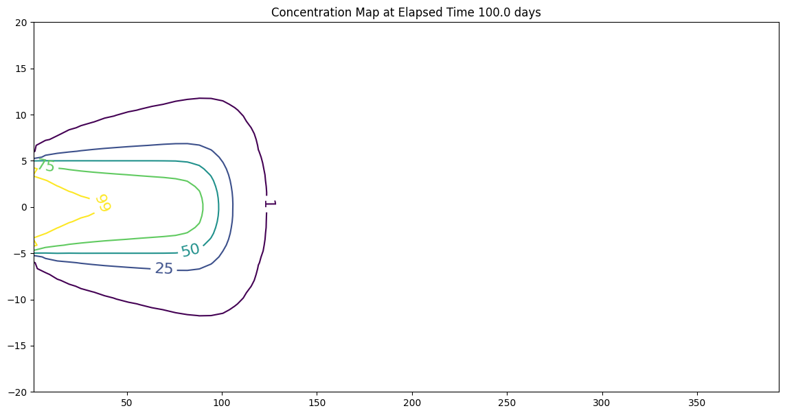
Construct 2D contour plots (equivalent to a profile plot)
# make a plot
x_max = 400
y_max = 20
# build a grid
nrows = 50
deltax = (x_max)/nrows
x = []
x.append(1)
for i in range(nrows):
    if x[i] == 0.0:
        x[i] = 0.00001
    x.append(x[i]+deltax)

ncols = 50
deltay = (y_max*2)/(ncols-1)
y = []
y.append(-y_max)
for i in range(1,ncols):
    if y[i-1] == 0.0:
        y[i-1] = 0.00001
    y.append(y[i-1]+deltay)

#y

#y = [i*deltay for i in range(how_many_points)] # constructor notation
#y[0]=0.001
ccc = [[0 for i in range(nrows)] for j in range(ncols)]

for jcol in range(ncols):
    for irow in range(nrows):
        ccc[irow][jcol] = c2ad(c_initial, x[irow], y[jcol], alphax, alphay, V, time, Y)

#y

my_xyz = [] # empty list
count=0
for irow in range(nrows):
    for jcol in range(ncols):
        my_xyz.append([ x[irow],y[jcol],ccc[irow][jcol] ])
       # print(count)
        count=count+1

#print(len(my_xyz))

import pandas
my_xyz = pandas.DataFrame(my_xyz) # convert into a data frame
import numpy
import matplotlib.pyplot
from scipy.interpolate import griddata
# extract lists from the dataframe
coord_x = my_xyz[0].values.tolist() # column 0 of dataframe
coord_y = my_xyz[1].values.tolist() # column 1 of dataframe
coord_z = my_xyz[2].values.tolist() # column 2 of dataframe
#print(min(coord_x), max(coord_x)) # activate to examine the dataframe
#print(min(coord_y), max(coord_y))
coord_xy = numpy.column_stack((coord_x, coord_y))
# Set plotting range in original data units
lon = numpy.linspace(min(coord_x), max(coord_x), 64)
lat = numpy.linspace(min(coord_y), max(coord_y), 64)
X, Y = numpy.meshgrid(lon, lat)
# Grid the data; use linear interpolation (choices are nearest, linear, cubic)
Z = griddata(numpy.array(coord_xy), numpy.array(coord_z), (X, Y), method='cubic')
# Build the map
fig, ax = matplotlib.pyplot.subplots()
fig.set_size_inches(14, 7)
CS = ax.contour(X, Y, Z, levels = [1,25,50,75,99])
ax.clabel(CS, inline=1, fontsize=16)
ax.set_title('Concentration Map at Elapsed Time '+ str(round(time,1))+' days');
Evaluate specific points