
Processing Texas Database
Following the process described in Prediction of Bridge Component Ratings Using Ordinal Logistic Regression Model but for Texas data.
import warnings
warnings.filterwarnings('ignore')
# Playing with Texas Data
local_file_name='2021TexasNBIData.csv'
import pandas as pd
# Read the NBI Database
texasdb = pd.read_csv(local_file_name)
# Verify the Structure
texasdb.describe()
| STATE_CODE_001 | ROUTE_PREFIX_005B | SERVICE_LEVEL_005C | DIRECTION_005E | HIGHWAY_DISTRICT_002 | COUNTY_CODE_003 | PLACE_CODE_004 | CRITICAL_FACILITY_006B | MIN_VERT_CLR_010 | KILOPOINT_011 | ... | FEDERAL_LANDS_105 | YEAR_RECONSTRUCTED_106 | PERCENT_ADT_TRUCK_109 | NATIONAL_NETWORK_110 | PIER_PROTECTION_111 | FUTURE_ADT_114 | YEAR_OF_FUTURE_ADT_115 | MIN_NAV_CLR_MT_116 | SUBMITTED_BY | DECK_AREA | |
|---|---|---|---|---|---|---|---|---|---|---|---|---|---|---|---|---|---|---|---|---|---|
| count | 64864.0 | 64861.000000 | 64863.000000 | 64802.000000 | 55179.000000 | 64864.000000 | 64864.000000 | 0.0 | 64864.000000 | 64627.000000 | ... | 55179.000000 | 55134.000000 | 64570.000000 | 64794.000000 | 1332.000000 | 55179.000000 | 55179.000000 | 654.000000 | 64864.000000 | 55179.000000 |
| mean | 48.0 | 3.308383 | 1.536192 | 0.055677 | 12.724932 | 241.292335 | 18365.083159 | NaN | 84.662018 | 14.325147 | ... | 0.001287 | 387.471143 | 9.593604 | 0.151573 | 1.081832 | 14738.009768 | 2032.348049 | 5.944190 | 48.065815 | 964.955676 |
| std | 0.0 | 1.524604 | 1.830507 | 0.409700 | 6.339940 | 148.401968 | 23984.559132 | NaN | 34.798024 | 81.534822 | ... | 0.066350 | 786.827517 | 10.983355 | 0.358609 | 0.389648 | 33669.125288 | 10.215096 | 52.747722 | 1.226490 | 2706.771529 |
| min | 48.0 | 1.000000 | 0.000000 | 0.000000 | 0.000000 | 1.000000 | 0.000000 | NaN | 0.000000 | 0.000000 | ... | 0.000000 | 0.000000 | 0.000000 | 0.000000 | 1.000000 | 0.000000 | 1900.000000 | 0.000000 | 48.000000 | 22.570000 |
| 25% | 48.0 | 2.000000 | 1.000000 | 0.000000 | 9.000000 | 113.000000 | 0.000000 | NaN | 99.990000 | 1.448000 | ... | 0.000000 | 0.000000 | 0.000000 | 0.000000 | 1.000000 | 500.000000 | 2033.000000 | 0.000000 | 48.000000 | 135.150000 |
| 50% | 48.0 | 3.000000 | 1.000000 | 0.000000 | 13.000000 | 201.000000 | 1000.000000 | NaN | 99.990000 | 6.437000 | ... | 0.000000 | 0.000000 | 6.000000 | 0.000000 | 1.000000 | 3510.000000 | 2033.000000 | 0.000000 | 48.000000 | 313.600000 |
| 75% | 48.0 | 4.000000 | 1.000000 | 0.000000 | 18.000000 | 373.000000 | 35000.000000 | NaN | 99.990000 | 19.195500 | ... | 0.000000 | 0.000000 | 14.000000 | 0.000000 | 1.000000 | 14000.000000 | 2034.000000 | 0.000000 | 48.000000 | 870.195000 |
| max | 48.0 | 8.000000 | 8.000000 | 4.000000 | 48.000000 | 507.000000 | 99315.000000 | NaN | 99.990000 | 9999.999000 | ... | 5.000000 | 2020.000000 | 99.000000 | 1.000000 | 5.000000 | 999999.000000 | 2086.000000 | 999.900000 | 75.000000 | 125732.720000 |
8 rows × 80 columns
Extract just culverts send to different object name (its probably just a HASH
We name our structure txculv (or whatever you want)
txculv = texasdb.loc[texasdb['STRUCTURE_TYPE_043B'] == 19]
txculv.describe()
| STATE_CODE_001 | ROUTE_PREFIX_005B | SERVICE_LEVEL_005C | DIRECTION_005E | HIGHWAY_DISTRICT_002 | COUNTY_CODE_003 | PLACE_CODE_004 | CRITICAL_FACILITY_006B | MIN_VERT_CLR_010 | KILOPOINT_011 | ... | FEDERAL_LANDS_105 | YEAR_RECONSTRUCTED_106 | PERCENT_ADT_TRUCK_109 | NATIONAL_NETWORK_110 | PIER_PROTECTION_111 | FUTURE_ADT_114 | YEAR_OF_FUTURE_ADT_115 | MIN_NAV_CLR_MT_116 | SUBMITTED_BY | DECK_AREA | |
|---|---|---|---|---|---|---|---|---|---|---|---|---|---|---|---|---|---|---|---|---|---|
| count | 20551.0 | 20551.00000 | 20551.000000 | 20551.000000 | 20545.000000 | 20551.000000 | 20551.000000 | 0.0 | 20551.000000 | 20551.000000 | ... | 20545.000000 | 20520.000000 | 20498.000000 | 20551.000000 | 190.000000 | 20545.000000 | 20545.000000 | 111.000000 | 20551.000000 | 20545.000000 |
| mean | 48.0 | 3.25916 | 1.343390 | 0.019123 | 12.900949 | 248.910759 | 15100.965111 | NaN | 99.702754 | 13.756241 | ... | 0.001898 | 583.425146 | 11.671675 | 0.077855 | 1.021053 | 11016.450961 | 2032.816938 | 6.052252 | 48.116247 | 219.712841 |
| std | 0.0 | 1.29903 | 1.492621 | 0.247959 | 6.490255 | 155.890098 | 23840.797409 | NaN | 5.223589 | 72.832328 | ... | 0.080438 | 904.383997 | 12.044279 | 0.267950 | 0.204652 | 28829.037024 | 7.714370 | 41.045256 | 1.674647 | 284.001639 |
| min | 48.0 | 1.00000 | 0.000000 | 0.000000 | 0.000000 | 1.000000 | 0.000000 | NaN | 0.000000 | 0.000000 | ... | 0.000000 | 0.000000 | 0.000000 | 0.000000 | 1.000000 | 1.000000 | 1900.000000 | 0.000000 | 48.000000 | 24.790000 |
| 25% | 48.0 | 3.00000 | 1.000000 | 0.000000 | 8.000000 | 113.000000 | 0.000000 | NaN | 99.990000 | 1.529000 | ... | 0.000000 | 0.000000 | 1.000000 | 0.000000 | 1.000000 | 530.000000 | 2033.000000 | 0.000000 | 48.000000 | 95.950000 |
| 50% | 48.0 | 3.00000 | 1.000000 | 0.000000 | 14.000000 | 231.000000 | 0.000000 | NaN | 99.990000 | 6.851000 | ... | 0.000000 | 0.000000 | 9.000000 | 0.000000 | 1.000000 | 2450.000000 | 2033.000000 | 0.000000 | 48.000000 | 149.410000 |
| 75% | 48.0 | 4.00000 | 1.000000 | 0.000000 | 18.000000 | 401.000000 | 27000.000000 | NaN | 99.990000 | 18.537000 | ... | 0.000000 | 1961.000000 | 18.000000 | 0.000000 | 1.000000 | 9030.000000 | 2033.000000 | 0.000000 | 48.000000 | 251.490000 |
| max | 48.0 | 8.00000 | 8.000000 | 4.000000 | 25.000000 | 507.000000 | 83745.000000 | NaN | 99.990000 | 9999.999000 | ... | 5.000000 | 2020.000000 | 90.000000 | 1.000000 | 3.000000 | 656470.000000 | 2052.000000 | 304.500000 | 74.000000 | 19993.960000 |
8 rows × 80 columns
list(texasdb)
['STATE_CODE_001',
 'STRUCTURE_NUMBER_008',
 'RECORD_TYPE_005A',
 'ROUTE_PREFIX_005B',
 'SERVICE_LEVEL_005C',
 'ROUTE_NUMBER_005D',
 'DIRECTION_005E',
 'HIGHWAY_DISTRICT_002',
 'COUNTY_CODE_003',
 'PLACE_CODE_004',
 'FEATURES_DESC_006A',
 'CRITICAL_FACILITY_006B',
 'FACILITY_CARRIED_007',
 'LOCATION_009',
 'MIN_VERT_CLR_010',
 'KILOPOINT_011',
 'BASE_HWY_NETWORK_012',
 'LRS_INV_ROUTE_013A',
 'SUBROUTE_NO_013B',
 'LAT_016',
 'LONG_017',
 'DETOUR_KILOS_019',
 'TOLL_020',
 'MAINTENANCE_021',
 'OWNER_022',
 'FUNCTIONAL_CLASS_026',
 'YEAR_BUILT_027',
 'TRAFFIC_LANES_ON_028A',
 'TRAFFIC_LANES_UND_028B',
 'ADT_029',
 'YEAR_ADT_030',
 'DESIGN_LOAD_031',
 'APPR_WIDTH_MT_032',
 'MEDIAN_CODE_033',
 'DEGREES_SKEW_034',
 'STRUCTURE_FLARED_035',
 'RAILINGS_036A',
 'TRANSITIONS_036B',
 'APPR_RAIL_036C',
 'APPR_RAIL_END_036D',
 'HISTORY_037',
 'NAVIGATION_038',
 'NAV_VERT_CLR_MT_039',
 'NAV_HORR_CLR_MT_040',
 'OPEN_CLOSED_POSTED_041',
 'SERVICE_ON_042A',
 'SERVICE_UND_042B',
 'STRUCTURE_KIND_043A',
 'STRUCTURE_TYPE_043B',
 'APPR_KIND_044A',
 'APPR_TYPE_044B',
 'MAIN_UNIT_SPANS_045',
 'APPR_SPANS_046',
 'HORR_CLR_MT_047',
 'MAX_SPAN_LEN_MT_048',
 'STRUCTURE_LEN_MT_049',
 'LEFT_CURB_MT_050A',
 'RIGHT_CURB_MT_050B',
 'ROADWAY_WIDTH_MT_051',
 'DECK_WIDTH_MT_052',
 'VERT_CLR_OVER_MT_053',
 'VERT_CLR_UND_REF_054A',
 'VERT_CLR_UND_054B',
 'LAT_UND_REF_055A',
 'LAT_UND_MT_055B',
 'LEFT_LAT_UND_MT_056',
 'DECK_COND_058',
 'SUPERSTRUCTURE_COND_059',
 'SUBSTRUCTURE_COND_060',
 'CHANNEL_COND_061',
 'CULVERT_COND_062',
 'OPR_RATING_METH_063',
 'OPERATING_RATING_064',
 'INV_RATING_METH_065',
 'INVENTORY_RATING_066',
 'STRUCTURAL_EVAL_067',
 'DECK_GEOMETRY_EVAL_068',
 'UNDCLRENCE_EVAL_069',
 'POSTING_EVAL_070',
 'WATERWAY_EVAL_071',
 'APPR_ROAD_EVAL_072',
 'WORK_PROPOSED_075A',
 'WORK_DONE_BY_075B',
 'IMP_LEN_MT_076',
 'DATE_OF_INSPECT_090',
 'INSPECT_FREQ_MONTHS_091',
 'FRACTURE_092A',
 'UNDWATER_LOOK_SEE_092B',
 'SPEC_INSPECT_092C',
 'FRACTURE_LAST_DATE_093A',
 'UNDWATER_LAST_DATE_093B',
 'SPEC_LAST_DATE_093C',
 'BRIDGE_IMP_COST_094',
 'ROADWAY_IMP_COST_095',
 'TOTAL_IMP_COST_096',
 'YEAR_OF_IMP_097',
 'OTHER_STATE_CODE_098A',
 'OTHER_STATE_PCNT_098B',
 'OTHR_STATE_STRUC_NO_099',
 'STRAHNET_HIGHWAY_100',
 'PARALLEL_STRUCTURE_101',
 'TRAFFIC_DIRECTION_102',
 'TEMP_STRUCTURE_103',
 'HIGHWAY_SYSTEM_104',
 'FEDERAL_LANDS_105',
 'YEAR_RECONSTRUCTED_106',
 'DECK_STRUCTURE_TYPE_107',
 'SURFACE_TYPE_108A',
 'MEMBRANE_TYPE_108B',
 'DECK_PROTECTION_108C',
 'PERCENT_ADT_TRUCK_109',
 'NATIONAL_NETWORK_110',
 'PIER_PROTECTION_111',
 'BRIDGE_LEN_IND_112',
 'SCOUR_CRITICAL_113',
 'FUTURE_ADT_114',
 'YEAR_OF_FUTURE_ADT_115',
 'MIN_NAV_CLR_MT_116',
 'FED_AGENCY',
 'SUBMITTED_BY',
 'BRIDGE_CONDITION',
 'LOWEST_RATING',
 'DECK_AREA']
txculv = txculv[['CULVERT_COND_062','YEAR_BUILT_027','ADT_029','DESIGN_LOAD_031','OPERATING_RATING_064','STRUCTURAL_EVAL_067',
                  'PERCENT_ADT_TRUCK_109','BRIDGE_CONDITION','YEAR_RECONSTRUCTED_106']].copy()
txculv.head()
| CULVERT_COND_062 | YEAR_BUILT_027 | ADT_029 | DESIGN_LOAD_031 | OPERATING_RATING_064 | STRUCTURAL_EVAL_067 | PERCENT_ADT_TRUCK_109 | BRIDGE_CONDITION | YEAR_RECONSTRUCTED_106 | |
|---|---|---|---|---|---|---|---|---|---|
| 0 | 7 | 2008 | 100.0 | 5 | 38.6 | 7 | 10.0 | G | 0.0 |
| 5 | 7 | 1990 | 15.0 | 0 | 36.3 | 7 | NaN | G | 0.0 |
| 18 | 7 | 1930 | 5581.0 | 0 | 32.7 | 6 | 16.0 | G | 1962.0 |
| 19 | 6 | 1934 | 5104.0 | 2 | 40.8 | 6 | 17.0 | F | 1959.0 |
| 21 | 6 | 1967 | 4348.0 | 5 | 44.4 | 6 | 19.0 | F | 0.0 |
txculv.describe()
| YEAR_BUILT_027 | ADT_029 | OPERATING_RATING_064 | PERCENT_ADT_TRUCK_109 | YEAR_RECONSTRUCTED_106 | |
|---|---|---|---|---|---|
| count | 20551.000000 | 20551.000000 | 20476.000000 | 20498.000000 | 20520.000000 |
| mean | 1969.900151 | 8578.712715 | 39.604732 | 11.671675 | 583.425146 |
| std | 25.511268 | 21636.892122 | 9.133697 | 12.044279 | 904.383997 |
| min | 1914.000000 | 0.000000 | 0.000000 | 0.000000 | 0.000000 |
| 25% | 1951.000000 | 400.000000 | 32.700000 | 1.000000 | 0.000000 |
| 50% | 1967.000000 | 1950.000000 | 44.400000 | 9.000000 | 0.000000 |
| 75% | 1990.000000 | 7101.500000 | 44.400000 | 18.000000 | 1961.000000 |
| max | 2020.000000 | 313693.000000 | 99.900000 | 90.000000 | 2020.000000 |
age = 2022 - txculv['YEAR_BUILT_027'] # age of culvert, surrogate for service life
drat = txculv['OPERATING_RATING_064'].fillna(1) # operating rating (in tons), nan is 1
drat = pd.to_numeric(drat) # coerce to numeric
steval = txculv['STRUCTURAL_EVAL_067'].fillna(1).replace('*','1') # structural eval, nan is 1 (not in original NBI coding tables)
steval = pd.to_numeric(steval) # coerce to numeric
adt =  txculv['ADT_029'].fillna(1) #
adt = pd.to_numeric(adt) # coerce to numeric
pctrk =  txculv['PERCENT_ADT_TRUCK_109'].fillna(txculv['PERCENT_ADT_TRUCK_109'].mean()) #
pctrk = pd.to_numeric(pctrk) # coerce to numeric


#df_filled2 = df.fillna(df.mean())
frame = { 'AGE': age, 'DRAT': drat, "ADT" :adt, "STEVAL":steval, "PCTRK":pctrk}
#frame = { 'AGE': age, 'DRAT': drat, "STEVAL":steval}
#Creating DataFrame by passing Dictionary
X = pd.DataFrame(frame)  # our design matrix
Now build our target
Prepare the target variable, from the culvert condition. The series has NaN and we convert these to a goofy string
pre_target = txculv['CULVERT_COND_062'].fillna('11').replace('N','10') # Nan to 11, "N" to 10 so all codes able to be numeric
print("Type ",type(pre_target[0]))
Type <class 'str'>
then convert from string to numeric.
pre_target = pd.to_numeric(pre_target)
print("Type ",type(pre_target[0]))
Type <class 'numpy.int64'>
Need a function to select the two conditions
def isok(value_int): # function to interpret condition rating and issue binary state 0 == fail 1 == OK
    cut = 3
    if value_int > cut:
        isok = 1
    elif value_int <= cut:
        isok = 0
    return(isok)

y = pre_target.apply(isok) # our target vector
Now check that our design matrix and target vector have correct structure
X.describe()
| AGE | DRAT | ADT | STEVAL | PCTRK | |
|---|---|---|---|---|---|
| count | 20551.000000 | 20551.000000 | 20551.000000 | 20551.000000 | 20551.000000 |
| mean | 52.099849 | 39.463846 | 8578.712715 | 6.164372 | 11.671675 |
| std | 25.511268 | 9.409530 | 21636.892122 | 0.838454 | 12.028738 |
| min | 2.000000 | 0.000000 | 0.000000 | 0.000000 | 0.000000 |
| 25% | 32.000000 | 32.700000 | 400.000000 | 6.000000 | 1.000000 |
| 50% | 55.000000 | 44.400000 | 1950.000000 | 6.000000 | 9.000000 |
| 75% | 71.000000 | 44.400000 | 7101.500000 | 7.000000 | 18.000000 |
| max | 108.000000 | 99.900000 | 313693.000000 | 9.000000 | 90.000000 |
y.describe()
count    20551.000000
mean         0.999465
std          0.023130
min          0.000000
25%          1.000000
50%          1.000000
75%          1.000000
max          1.000000
Name: CULVERT_COND_062, dtype: float64
# Now we can do some machine learning
# split X and y into training and testing sets
from sklearn.model_selection import train_test_split
X_train,X_test,y_train,y_test=train_test_split(X,y,test_size=0.25,random_state=0)
# import the class
from sklearn.linear_model import LogisticRegression

# instantiate the model (using the default parameters)
#logreg = LogisticRegression()
logreg = LogisticRegression()
# fit the model with data
logreg.fit(X_train,y_train)

#
y_pred=logreg.predict(X_test)
print(logreg.intercept_[0])
print(logreg.coef_)
#y.head()
0.08278239586830166
[[-1.03778439e-02 -1.30938676e-01  6.65067052e-05  2.17738437e+00
   6.97735441e-01]]
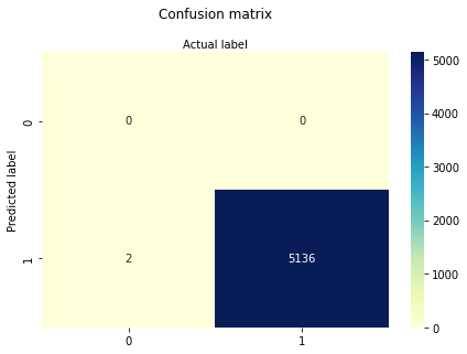
# import the metrics class
from sklearn import metrics
cnf_matrix = metrics.confusion_matrix(y_pred, y_test)
cnf_matrix
import matplotlib.pyplot as plt
import numpy as np
import seaborn as sns
import pandas as pd
class_names=[0,1] # name  of classes
fig, ax = plt.subplots()
tick_marks = np.arange(len(class_names))
plt.xticks(tick_marks, class_names)
plt.yticks(tick_marks, class_names)
# create heatmap
sns.heatmap(pd.DataFrame(cnf_matrix), annot=True, cmap="YlGnBu" ,fmt='g')
ax.xaxis.set_label_position("top")
plt.tight_layout()
plt.title('Confusion matrix', y=1.1)
plt.ylabel('Predicted label')
plt.xlabel('Actual label');
# import the class
from sklearn.linear_model import PoissonRegressor

# instantiate the model (using the default parameters)
#logreg = LogisticRegression()
posreg = PoissonRegressor()
# fit the model with data
posreg.fit(X_train,y_train)

#
y_pred=posreg.predict(X_test)
print(posreg.intercept_)
print(posreg.coef_)
#y.head()
-0.0005840932119201926
[0. 0. 0. 0. 0.]
y_pred
array([0.99941608, 0.99941608, 0.99941608, ..., 0.99941608, 0.99941608,
       0.99941608])
Structurally Deficient (SD): This term was previously defined in https://www.fhwa.dot.gov/bridge/0650dsup.cfm as having a condition rating of 4 or less for Item 58 (Deck), Item 59 (Superstructure), Item 60 (Substructure), or Item 62 (Culvert), OR having an appraisal rating of 2 or less for Item 67 (Structural Condition) or Item 71 (Waterway Adequacy) Beginning with the 2018 data archive, this term will be defined in accordance with the Pavement and Bridge Condition Performance Measures final rule, published in January of 2017, as a classification given to a bridge which has any component [Item 58, 59, 60, or 62] in Poor or worse condition [code of 4 or less].
This capacity rating, referred to as the operating rating, will result in the absolute maximum permissible load level to which the structure may be subjected for the vehicle type used in the rating. Code the operating rating as a 3-digit number to represent the total mass in metric tons of the entire vehicle measured to the nearest tenth of a metric ton (with an assumed decimal point).
#type(pre_target[0])
Prepare the target variable, the culvert condition as above (not processing just yet). The series has NaN and we convert these to a goofy string then convert from string to numeric.
Now make a proper target
#target