
Unsupervised Learning
topic
Note
In unsupervised learning, the dataset is a collection of unlabeled examples \({x_i}_{i=1}^N\) Each element (column) of \(x_i\) is called a feature vector, or in my jargon a predictor.
The goal of an unsupervised learner is to produce a model (aka fitted hypothesis) that will take as input a feature vector and produce as output another vector or a value that can be used to solve a practical problem - usually the output is some kind of pattern recognition that can be further leveraged. For example in clustering the output is an ID of a cluster (pattern) for the various features; in dimensionality reduction the output is a feature vector with fewer features, in outlier detection the output might me some measure of how far from the others a particular “row” in the dataset is.
What follows below is lifted largely from IBM marketing materials - its kind of fluffy but worth a read as we construct a language relevant to ML in Civil Engineering
What is unsupervised learning?
Unsupervised learning uses algorithms to analyze and cluster unlabeled datasets. These algorithms discover patterns or data groupings without the need for human intervention. Its ability to discover similarities and differences in information make it the ideal solution for exploratory data analysis, cross-selling strategies, customer segmentation, and image recognition.
Common unsupervised learning approaches
Unsupervised learning models are utilized for three main tasks—clustering, association, and dimensionality reduction. Below we’ll define each learning method and highlight common algorithms and approaches to conduct them effectively.
Clustering
Clustering is a data mining technique which groups unlabeled data based on their similarities or differences. Clustering algorithms are used to process raw, unclassified data objects into groups represented by structures or patterns in the information. Clustering algorithms can be categorized into a few types, specifically exclusive, overlapping, hierarchical, and probabilistic.
Exclusive and Overlapping Clustering
Exclusive clustering is a form of grouping that stipulates a data point can exist only in one cluster. This can also be referred to as “hard” clustering. The K-means clustering algorithm is an example of exclusive clustering.
K-means clustering is a common example of an exclusive clustering method where data points are assigned into K groups, where K represents the number of clusters based on the distance from each group’s centroid. The data points closest to a given centroid will be clustered under the same category. A larger K value will be indicative of smaller groupings with more granularity whereas a smaller K value will have larger groupings and less granularity. K-means clustering is commonly used in market segmentation, document clustering, image segmentation, and image compression.
Overlapping clusters differs from exclusive clustering in that it allows data points to belong to multiple clusters with separate degrees of membership. “Soft” or fuzzy k-means clustering is an example of overlapping clustering.
Hierarchical clustering
Hierarchical clustering, also known as hierarchical cluster analysis (HCA), is an unsupervised clustering algorithm that can be categorized in two ways; they can be agglomerative or divisive. Agglomerative clustering is considered a “bottoms-up approach.” Its data points are isolated as separate groupings initially, and then they are merged together iteratively on the basis of similarity until one cluster has been achieved. Four different methods are commonly used to measure similarity:
Ward’s linkage: This method states that the distance between two clusters is defined by the increase in the sum of squared after the clusters are merged.
Average linkage: This method is defined by the mean distance between two points in each cluster
Complete (or maximum) linkage: This method is defined by the maximum distance between two points in each cluster
Single (or minimum) linkage: This method is defined by the minimum distance between two points in each cluster
Euclidean distance is the most common metric used to calculate these distances; however, other metrics, such as Manhattan distance, are also cited in clustering literature.
Divisive clustering can be defined as the opposite of agglomerative clustering; instead it takes a “top-down” approach. In this case, a single data cluster is divided based on the differences between data points. Divisive clustering is not commonly used, but it is still worth noting in the context of hierarchical clustering. These clustering processes are usually visualized using a dendrogram, a tree-like diagram that documents the merging or splitting of data points at each iteration. Diagram of a dendrogram
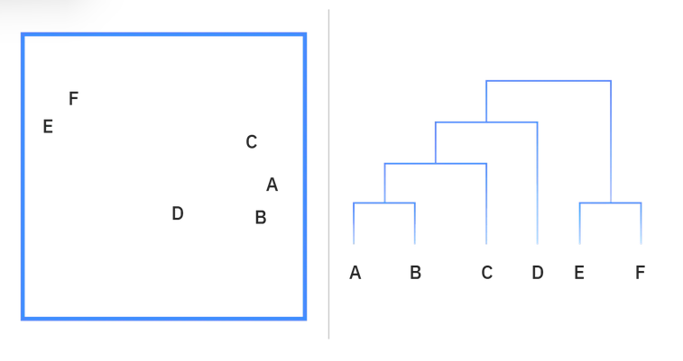
Diagram of a Dendrogram; reading the chart “bottom-up” demonstrates agglomerative clustering while “top-down” is indicative of divisive clustering
Probabilistic clustering
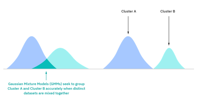
A probabilistic model is an unsupervised technique that helps us solve density estimation or “soft” clustering problems. In probabilistic clustering, data points are clustered based on the likelihood that they belong to a particular distribution. The Gaussian Mixture Model (GMM) is the one of the most commonly used probabilistic clustering methods.
Gaussian Mixture Models are classified as mixture models, which means that they are made up of an unspecified number of probability distribution functions. GMMs are primarily leveraged to determine which Gaussian, or normal, probability distribution a given data point belongs to. If the mean or variance are known, then we can determine which distribution a given data point belongs to. However, in GMMs, these variables are not known, so we assume that a latent, or hidden, variable exists to cluster data points appropriately. While it is not required to use the Expectation-Maximization (EM) algorithm, it is a commonly used to estimate the assignment probabilities for a given data point to a particular data cluster.
Before and after illustration of distribution models for Gaussian Mixture Models
Association Rules
An association rule is a rule-based method for finding relationships between variables in a given dataset. These methods are frequently used for market basket analysis, allowing companies to better understand relationships between different products. Understanding consumption habits of customers enables businesses to develop better cross-selling strategies and recommendation engines. Examples of this can be seen in Amazon’s “Customers Who Bought This Item Also Bought” or Spotify’s “Discover Weekly” playlist. While there are a few different algorithms used to generate association rules, such as Apriori, Eclat, and FP-Growth, the Apriori algorithm is most widely used.
Apriori algorithms
Apriori algorithms have been popularized through market basket analyses, leading to different recommendation engines for music platforms and online retailers. They are used within transactional datasets to identify frequent itemsets, or collections of items, to identify the likelihood of consuming a product given the consumption of another product. For example, if I play Black Sabbath’s radio on Spotify, starting with their song “Orchid”, one of the other songs on this channel will likely be a Led Zeppelin song, such as “Over the Hills and Far Away.” This is based on my prior listening habits as well as the ones of others. Apriori algorithms use a hash tree to count itemsets, navigating through the dataset in a breadth-first manner.
Dimensionality reduction
While more data generally yields more accurate results, it can also impact the performance of machine learning algorithms (e.g. overfitting) and it can also make it difficult to visualize datasets. Dimensionality reduction is a technique used when the number of features, or dimensions, in a given dataset is too high. It reduces the number of data inputs to a manageable size while also preserving the integrity of the dataset as much as possible. It is commonly used in the preprocessing data stage, and there are a few different dimensionality reduction methods that can be used, such as:
Principal component analysis
Principal component analysis (PCA) is a type of dimensionality reduction algorithm which is used to reduce redundancies and to compress datasets through feature extraction. This method uses a linear transformation to create a new data representation, yielding a set of “principal components.” The first principal component is the direction which maximizes the variance of the dataset. While the second principal component also finds the maximum variance in the data, it is completely uncorrelated to the first principal component, yielding a direction that is perpendicular, or orthogonal, to the first component. This process repeats based on the number of dimensions, where a next principal component is the direction orthogonal to the prior components with the most variance.
Singular value decomposition
Singular value decomposition (SVD) is another dimensionality reduction approach which factorizes a matrix, A, into three, low-rank matrices. SVD is denoted by the formula, A = USVT, where U and V are orthogonal matrices. S is a diagonal matrix, and S values are considered singular values of matrix A. Similar to PCA, it is commonly used to reduce noise and compress data, such as image files.
Autoencoders
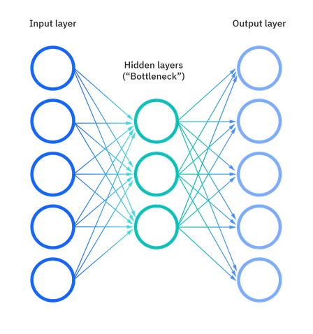
Autoencoders leverage neural networks to compress data and then recreate a new representation of the original data’s input. Looking at the image below, you can see that the hidden layer specifically acts as a bottleneck to compress the input layer prior to reconstructing within the output layer. The stage from the input layer to the hidden layer is referred to as “encoding” while the stage from the hidden layer to the output layer is known as “decoding.”
Example Applications
Machine learning techniques have become a common method to improve a product user experience and to test systems for quality assurance. Unsupervised learning provides an exploratory path to view data, allowing businesses to identify patterns in large volumes of data more quickly when compared to manual observation. Some of the most common real-world applications of unsupervised learning are:
News Sections: Google News uses unsupervised learning to categorize articles on the same story from various online news outlets. For example, the results of a presidential election could be categorized under their label for “US” news.
Computer vision: Unsupervised learning algorithms are used for visual perception tasks, such as object recognition.
Medical imaging: Unsupervised machine learning provides essential features to medical imaging devices, such as image detection, classification and segmentation, used in radiology and pathology to diagnose patients quickly and accurately.
Anomaly detection: Unsupervised learning models can comb through large amounts of data and discover atypical data points within a dataset. These anomalies can raise awareness around faulty equipment, human error, or breaches in security.
Customer personas: Defining customer personas makes it easier to understand common traits and business clients’ purchasing habits. Unsupervised learning allows businesses to build better buyer persona profiles, enabling organizations to align their product messaging more appropriately.
Recommendation Engines: Using past purchase behavior data, unsupervised learning can help to discover data trends that can be used to develop more effective cross-selling strategies. This is used to make relevant add-on recommendations to customers during the checkout process for online retailers.
Unsupervised vs. supervised learning
Supervised learning algorithms use labeled data. From that data, it either predicts future outcomes or assigns data to specific categories based on the regression or classification engine that is applied. Supervised learning algorithms tend to be more accurate than unsupervised learning models, but they require upfront human interaction to label the data appropriately. However, these labelled datasets allow supervised learning algorithms to function with smaller training sets to produce intended outcomes. Common regression and classification techniques are linear and logistic regression, naïve bayes, KNN algorithm, and random forest.
Challenges of unsupervised learning
While unsupervised learning has many benefits, some challenges can occur when it allows machine learning models to execute without any human intervention. Some of these challenges can include:
Computational complexity due to a high volume of training data
Longer training times
Higher risk of inaccurate results
Human intervention to validate output variables
lorem ipsum
References
Chan, Jamie. Machine Learning With Python For Beginners: A Step-By-Step Guide with Hands-On Projects (Learn Coding Fast with Hands-On Project Book 7) (p. 2). Kindle Edition.