Prediction Engines
This section examines the process of prediction, or forecasting if you will. In prediction we are attempting to build an excitation-response model so that when new (future) excitations are supplied to the model, the new (future) responses are predicted.
As an example, suppose a 1 Newton force is applied to a 1 kilogram object, we expect an acceleration of 1 meter per second per second. The inputs are mass and force, the response is acceleration. Now if we triple the mass, and leave the force unchanged then the acceleration is predicted to be 1/3 meter per second per second. The prediction machine structure in this example could be something like
After training the fitted (learned) model would determine that \(\beta_1=\beta_2=\beta_3=1\) and \(\beta_4=-1\) is the best performing model and that would be our prediction engine.
Or we could just trust Newton that the prediction model is
A Simple Prediction Machine
Imagine a basic machine that takes a question, does some “thinking” and pushes out an answer. Here’s a diagram of the process:

Computers don’t really think, they’re just fast calculators (actually difference engines, but that’s for another time), so let’s use more appropriate words to describe what’s going on:
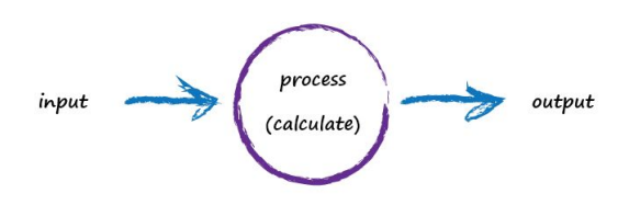
A computer takes some input, does some calculation and poops out an output. The following illustrates this. An input of “3 x 4” is processed, perhaps by turning multiplication into an easier set of additions, and the output answer “12” poops out.
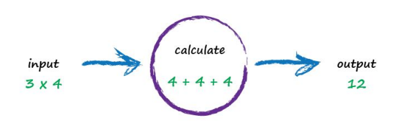
Not particularly impressive - we could even write a function!
def threeByfour(a,b):
    value = a * b
    return(value)

a = 3; b=4

print('a times b =',threeByfour(a,b))
a times b = 12
Next, Imagine a machine that converts kilometres to miles, like the following:
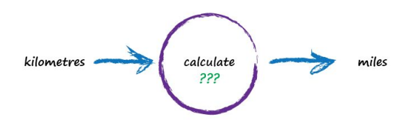
But imagine we don’t know the formula for converting between kilometres and miles. All we know is the the relationship between the two is linear. That means if we double the number in miles, the same distance in kilometres is also doubled.
This linear relationship between kilometres and miles gives us a clue about that mysterious calculation it needs to be of the form “miles = kilometres x c”, where c is a constant. We don’t know what this constant c is yet. The only other clues we have are some examples pairing kilometres with the correct value for miles. These are like real world observations used to test scientific theories - they’re examples of real world truth.
Truth Example |
Kilometres |
Miles |
|---|---|---|
1 |
0 |
0 |
2 |
100 |
62.137 |
To work out that missing constant c just pluck a value at random and give it a try! Let’s try c = 0.5 and see what happens.
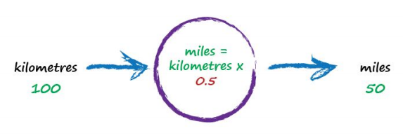
Here we have miles = kilometres x c, where kilometres is 100 and c is our current guess at 0.5. That gives 50 miles. Okay. That’s not bad at all given we chose c = 0.5 at random! But we know it’s not exactly right because our truth example number 2 tells us the answer should be 62.137. We’re wrong by 12.137. That’s the error, the difference between our calculated answer and the actual truth from our list of examples. That is,
error = truth - calculated = 62.137 - 50 = 12.137
def km2miles(km,c):
    value = km*c
    return(value)

x=100
c=0.5
y=km2miles(x,c)
t=62.137

print(x, 'kilometers is estimated to be ',y,' miles')
print('Estimation error is ', t-y , 'miles')
100 kilometers is estimated to be  50.0  miles
Estimation error is  12.137 miles
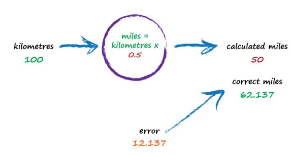
So what next? We know we’re wrong, and by how much. Instead of being a reason to despair, we use this error to guide a second, better, guess at c. Look at that error again. We were short by 12.137. Because the formula for converting kilometres to miles is linear, miles = kilometres x c, we know that increasing c will increase the output. Let’s nudge c up from 0.5 to 0.6 and see what happens.

With c now set to 0.6, we get miles = kilometres x c = 100 x 0.6 = 60. That’s better than the previous answer of 50. We’re clearly making progress! Now the error is a much smaller 2.137. It might even be an error we’re happy to live with.
def km2miles(km,c):
    value = km*c
    return(value)

x=100
c=0.6
y=km2miles(x,c)
t=62.137

print(x, 'kilometers is estimated to be ',y,' miles')
print('Estimation error is ', t-y , 'miles')
100 kilometers is estimated to be  60.0  miles
Estimation error is  2.1370000000000005 miles
The important point here is that we used the error to guide how we nudged the value of c. We wanted to increase the output from 50 so we increased c a little bit. Rather than try to use algebra to work out the exact amount c needs to change, let’s continue with this approach of refining c. If you’re not convinced, and think it’s easy enough to work out the exact answer, remember that many more interesting problems won’t have simple mathematical formulas relating the output and input. That’s why we use “machine learning” methods. Let’s do this again. The output of 60 is still too small. Let’s nudge the value of c up again from 0.6 to 0.7.
def km2miles(km,c):
    value = km*c
    return(value)

x=100
c=0.7
y=km2miles(x,c)
t=62.137

print(x, 'kilometers is estimated to be ',y,' miles')
print('Estimation error is ', t-y , 'miles')
100 kilometers is estimated to be  70.0  miles
Estimation error is  -7.8629999999999995 miles
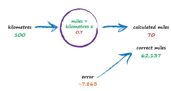
Oh no! We’ve gone too far and overshot the known correct answer. Our previous error was 2.137 but now it’s -7.863. The minus sign simply says we overshot rather than undershot, remember the error is (correct value - calculated value). Ok so c = 0.6 was way better than c = 0.7. We could be happy with the small error from c = 0.6 and end this exercise now. But let’s go on for just a bit longer.
Let’s split the difference from our last guess - we still have overshot, but not as much (-2.8629).
Split again to c=0.625, and overshoot is only (-0.3629) (we could sucessively split the c values until we are close enough. The method just illustrated is called bisection, and the important point is that we avoided any mathematics other than bigger/smaller and multiplication and subtraction; hence just arithmetic.)
That’s much much better than before. We have an output value of 62.5 which is only wrong by 0.3629 from the correct 62.137. So that last effort taught us that we should moderate how much we nudge the value of c. If the outputs are getting close to the correct answer - that is, the error is getting smaller - then don’t nudge the constant so much. That way we avoid overshooting the right value, like we did earlier. Again without getting too distracted by exact ways of working out c, and to remain focussed on this idea of successively refining it, we could suggest that the correction is a fraction of the error. That’s intuitively right - a big error means a bigger correction is needed, and a tiny error means we need the teeniest of nudges to c. What we’ve just done, believe it or not, is walked through the very core process of learning in a neural network - we’ve trained the machine to get better and better at giving the right answer. It is worth pausing to reflect on that - we’ve not solved a problem exactly in one step. Instead, we’ve taken a very different approach by trying an answer and improving it repeatedly. Some use the term iterative and it means repeatedly improving an answer bit by bit.
def km2miles(km,c):
    value = km*c
    return(value)

x=100
c=0.65
y=km2miles(x,c)
t=62.137

print(x, 'kilometers is estimated to be ',y,' miles')
print('Estimation error is ', t-y , 'miles')
100 kilometers is estimated to be  65.0  miles
Estimation error is  -2.8629999999999995 miles
def km2miles(km,c):
    value = km*c
    return(value)

x=100
c=0.625
y=km2miles(x,c)
t=62.137

print(x, 'kilometers is estimated to be ',y,' miles')
print('Estimation error is ', t-y , 'miles')
100 kilometers is estimated to be  62.5  miles
Estimation error is  -0.36299999999999955 miles
Now let’s automate the process.
We have our prediction engine structure embedded into the km2miles() function. We have a database of observations (albeit its kind of small). We need to find a value of c that’s good enough then we can use the prediction engine to convert new values. As stated above bisection seems appropriate, so here we will adapt a classical bisection algorithm for our machine.
Note
The code below is shamelessly lifted from Qingkai Kong, Timmy Siauw, Alexandre M. Bayen, 2021 Python Programming and Numerical Methods, Academic Press and adapted explicitly for the machine described herein. If you go to the source the authors use lambda objects to generalize their scripts, but I choose to simply break their fine programming structure for my needs; something everyone should get comfortable with.
def km2miles(km,c):
    value = km*c
    return(value)

howmany = 50 # number of iterations
clow = 0 # lower limit for c
chigh = 1 # upper limit for c
x=100 # ground truth value
dtrue = 62.137 # ground truth value
tol = 1e-6 # desired accuracy

import numpy # useful library with absolute value and sign functions

############ Learning Phase ################
# check if clow and chigh bound a solution
if numpy.sign(km2miles(x,clow)-dtrue) == numpy.sign(km2miles(x,chigh)-dtrue):
    raise Exception("The scalars clow and chigh do not bound a solution")


for iteration in range(howmany):
# get midpoint
    m = (clow + chigh)/2

    if numpy.abs(km2miles(x,clow)-dtrue) < tol:
        # stopping condition, report m as root
        print('Normal Exit Learning Complete')
        break
    elif numpy.sign(km2miles(x,clow)-dtrue) == numpy.sign(km2miles(x,m)-dtrue):
        # case where m is an improvement on a.
        # Make recursive call with a = m
        clow = m # update a with m
    elif numpy.sign(km2miles(x,chigh)-dtrue) == numpy.sign(km2miles(x,m)-dtrue):
        # case where m is an improvement on b.
        # Make recursive call with b = m
        chigh = m # update b with m
####################################################
Normal Exit Learning Complete
############# Testing Phase ########################
y=km2miles(x,m)
print('number trials',iteration)
print('model c value',m)
print(x,'kilometers is estimated to be ',round(y,3),' miles')
print('Estimation error is ', round(dtrue-y,3) , 'miles')
print('Testing Complete')
number trials 27
model c value 0.6213699989020824
100 kilometers is estimated to be  62.137  miles
Estimation error is  0.0 miles
Testing Complete
############ Deployment Phase #######################
xx = 1000
y=km2miles(xx,m)
print(xx,'kilometers is estimated to be ',round(y,3),' miles')
1000 kilometers is estimated to be 621.37 miles
Learning Theory Concepts
Learning in the limit Given a continuous stream of examples where the learner predicts whether each one is a member of the concept or not and is then is told the correct answer, does the learner eventually converge to a correct concept and never make a mistake again. One can think of this as if the learner has a big enough training set, then it eventually can achieve a “perfect” fit. I am extrapolating a bit, but the idea is that in the limit perfection is achievable.
By simple enumeration (what I called Grid Search), concepts from any known finite hypothesis space are learnable in the limit, although typically requires an exponential (or doubly exponential) number of examples and time.
Recall my definitions:
Hypothesis is a structural representation of predictor response relationship; \(r=f(p)\)
Model is a fitted hypothesis. \(f(p) = \beta_1 p^{beta_2}\) where \(\beta_1\) and \(\beta_2\) have been determined by application of a learner (i.e. they are known). So all we do is supply predictor values and get a response.
Learner is an algorithm that fits a hypothesis to produce a data model.
Types of learners
Consistent Learner A learner L using a hypothesis H and training data D is said to be a consistent learner if it always outputs a model with zero error on D whenever H contains such a hypothesis. By definition, a consistent learner must produce a model in the version space for H given D.
Halving learner I cannot find a simple translation, its the name given to a concept where the learner splits the training data space into a partion that produces crappy models and a partition that produces good models or even consistent models (using above definition). I think the concept refers to the entire hypothesis,training,model process; obviously the ability to split the predictor space into the parts that are effective and not will be quite useful.
Ellipsoid learner Refers to a classification algorithm that searches an n-dimensional ellipsoid in the training domain to determine a classification scheme.
References
Chan, Jamie. Machine Learning With Python For Beginners: A Step-By-Step Guide with Hands-On Projects (Learn Coding Fast with Hands-On Project Book 7) (p. 2). Kindle Edition.
Rashid, Tariq. Make Your Own Neural Network. Kindle Edition.
