
Logistic Regression¶

For the last few sessions we have talked about simple linear regression …

We discussed …
The theory and implementation of simple linear regression in Python
OLS and MLE methods for estimation of slope and intercept coefficients
Errors (Noise, Variance, Bias) and their impacts on model’s performance
Confidence and prediction intervals
And Multiple Linear Regressions

What if we want to predict a discrete variable?
The general idea behind our efforts was to use a set of observed events (samples) to capture the relationship between one or more predictor (AKA input, indipendent) variables and an output (AKA response, dependent) variable. The nature of the dependent variables differentiates regression and classification problems.
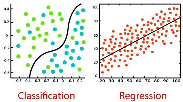
Regression problems have continuous and usually unbounded outputs. An example is when you’re estimating the salary as a function of experience and education level. Or all the examples we have covered so far!
On the other hand, classification problems have discrete and finite outputs called classes or categories. For example, predicting if an employee is going to be promoted or not (true or false) is a classification problem. There are two main types of classification problems:
Binary or binomial classification:
exactly two classes to choose between (usually 0 and 1, true and false, or positive and negative)
Multiclass or multinomial classification:
three or more classes of the outputs to choose from
When Do We Need Classification?
We can apply classification in many fields of science and technology. For example, text classification algorithms are used to separate legitimate and spam emails, as well as positive and negative comments. Other examples involve medical applications, biological classification, credit scoring, and more.
Logistic Regression¶
What is logistic regression? Logistic regression is a fundamental classification technique. It belongs to the group of linear classifiers and is somewhat similar to polynomial and linear regression. Logistic regression is fast and relatively uncomplicated, and it’s convenient for users to interpret the results. Although it’s essentially a method for binary classification, it can also be applied to multiclass problems.

Logistic regression is a statistical method for predicting binary classes. The outcome or target variable is dichotomous in nature. Dichotomous means there are only two possible classes. For example, it can be used for cancer detection problems. It computes the probability of an event occurrence. Logistic regression can be considered a special case of linear regression where the target variable is categorical in nature. It uses a log of odds as the dependent variable. Logistic Regression predicts the probability of occurrence of a binary event utilizing a logit function. HOW?
Remember the general format of the multiple linear regression model:
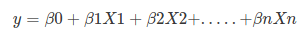
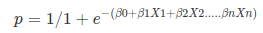
Where, y is dependent variable and x1, x2 … and Xn are explanatory variables. This was, as you know by now, a linear function. There is another famous function known as the Sigmoid Function, also called logistic function. Here is the equation for the Sigmoid function:
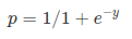
This image shows the sigmoid function (or S-shaped curve) of some variable 𝑥:
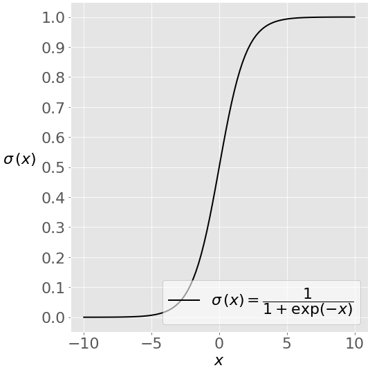
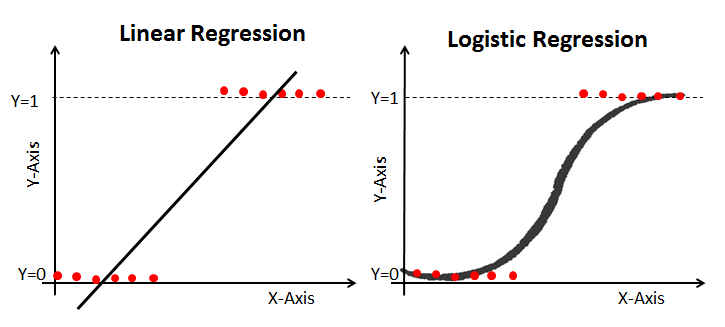
As you see, The sigmoid function has values very close to either 0 or 1 across most of its domain. It can take any real-valued number and map it into a value between 0 and 1. If the curve goes to positive infinity, y predicted will become 1, and if the curve goes to negative infinity, y predicted will become 0. This fact makes it suitable for application in classification methods since we are dealing with two discrete classes (labels, categories, …). If the output of the sigmoid function is more than 0.5, we can classify the outcome as 1 or YES, and if it is less than 0.5, we can classify it as 0 or NO. This cutoff value (threshold) is not always fixed at 0.5. If we apply the Sigmoid function on linear regression:
Notice the difference between linear regression and logistic regression:
logistic regression is estimated using Maximum Likelihood Estimation (MLE) approach. Maximizing the likelihood function determines the parameters that are most likely to produce the observed data.
Let’s work on an example in Python!
Diagnosing Diabetes
¶

The “diabetes.csv” dataset is originally from the National Institute of Diabetes and Digestive and Kidney Diseases. The objective of the dataset is to diagnostically predict whether or not a patient has diabetes, based on certain diagnostic measurements included in the dataset. Several constraints were placed on the selection of these instances from a larger database. In particular, all patients here are females at least 21 years old of Pima Indian heritage.
The datasets consists of several medical predictor variables and one target variable, Outcome. Predictor variables includes the number of pregnancies the patient has had, their BMI, insulin level, age, and so on.
Columns |
Info. |
|---|---|
Pregnancies |
Number of times pregnant |
Glucose |
Plasma glucose concentration a 2 hours in an oral glucose tolerance test |
BloodPressure |
Diastolic blood pressure (mm Hg) |
SkinThickness |
Triceps skin fold thickness (mm) |
Insulin |
2-Hour serum insulin (mu U/ml) |
BMI |
Body mass index (weight in kg/(height in m)^2) |
Diabetes pedigree |
Diabetes pedigree function |
Age |
Age (years) |
Outcome |
Class variable (0 or 1) 268 of 768 are 1, the others are 0 |
Let’s see if we can build a logistic regression model to accurately predict whether or not the patients in the dataset have diabetes or not? Acknowledgements: Smith, J.W., Everhart, J.E., Dickson, W.C., Knowler, W.C., & Johannes, R.S. (1988). Using the ADAP learning algorithm to forecast the onset of diabetes mellitus. In Proceedings of the Symposium on Computer Applications and Medical Care (pp. 261–265). IEEE Computer Society Press.
import numpy as np
import pandas as pd
from matplotlib import pyplot as plt
import sklearn.metrics as metrics
import seaborn as sns
%matplotlib inline
# Import the dataset:
data = pd.read_csv("diabetes.csv")
data.rename(columns = {'Pregnancies':'pregnant', 'Glucose':'glucose','BloodPressure':'bp','SkinThickness':'skin',
                       'Insulin	':'Insulin','BMI':'bmi','DiabetesPedigreeFunction':'pedigree','Age':'age',
                              'Outcome':'label'}, inplace = True)
data.head()
| pregnant | glucose | bp | skin | Insulin | bmi | pedigree | age | label | |
|---|---|---|---|---|---|---|---|---|---|
| 0 | 6 | 148 | 72 | 35 | 0 | 33.6 | 0.627 | 50 | 1 |
| 1 | 1 | 85 | 66 | 29 | 0 | 26.6 | 0.351 | 31 | 0 |
| 2 | 8 | 183 | 64 | 0 | 0 | 23.3 | 0.672 | 32 | 1 |
| 3 | 1 | 89 | 66 | 23 | 94 | 28.1 | 0.167 | 21 | 0 |
| 4 | 0 | 137 | 40 | 35 | 168 | 43.1 | 2.288 | 33 | 1 |
data.describe()
| pregnant | glucose | bp | skin | Insulin | bmi | pedigree | age | label | |
|---|---|---|---|---|---|---|---|---|---|
| count | 768.000000 | 768.000000 | 768.000000 | 768.000000 | 768.000000 | 768.000000 | 768.000000 | 768.000000 | 768.000000 |
| mean | 3.845052 | 120.894531 | 69.105469 | 20.536458 | 79.799479 | 31.992578 | 0.471876 | 33.240885 | 0.348958 |
| std | 3.369578 | 31.972618 | 19.355807 | 15.952218 | 115.244002 | 7.884160 | 0.331329 | 11.760232 | 0.476951 |
| min | 0.000000 | 0.000000 | 0.000000 | 0.000000 | 0.000000 | 0.000000 | 0.078000 | 21.000000 | 0.000000 |
| 25% | 1.000000 | 99.000000 | 62.000000 | 0.000000 | 0.000000 | 27.300000 | 0.243750 | 24.000000 | 0.000000 |
| 50% | 3.000000 | 117.000000 | 72.000000 | 23.000000 | 30.500000 | 32.000000 | 0.372500 | 29.000000 | 0.000000 |
| 75% | 6.000000 | 140.250000 | 80.000000 | 32.000000 | 127.250000 | 36.600000 | 0.626250 | 41.000000 | 1.000000 |
| max | 17.000000 | 199.000000 | 122.000000 | 99.000000 | 846.000000 | 67.100000 | 2.420000 | 81.000000 | 1.000000 |
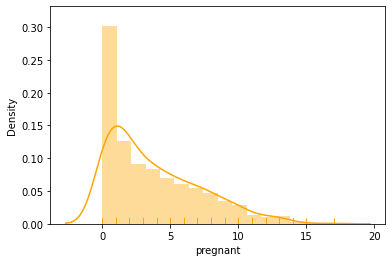
#Check some histograms
sns.distplot(data['pregnant'], kde = True, rug= True, color ='orange')
/opt/jupyterhub/lib/python3.8/site-packages/seaborn/distributions.py:2619: FutureWarning: `distplot` is a deprecated function and will be removed in a future version. Please adapt your code to use either `displot` (a figure-level function with similar flexibility) or `histplot` (an axes-level function for histograms).
  warnings.warn(msg, FutureWarning)
/opt/jupyterhub/lib/python3.8/site-packages/seaborn/distributions.py:2103: FutureWarning: The `axis` variable is no longer used and will be removed. Instead, assign variables directly to `x` or `y`.
  warnings.warn(msg, FutureWarning)
<AxesSubplot:xlabel='pregnant', ylabel='Density'>
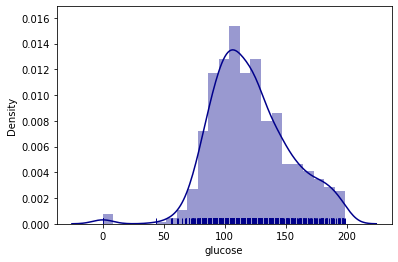
sns.distplot(data['glucose'], kde = True, rug= True, color ='darkblue')
/opt/jupyterhub/lib/python3.8/site-packages/seaborn/distributions.py:2619: FutureWarning: `distplot` is a deprecated function and will be removed in a future version. Please adapt your code to use either `displot` (a figure-level function with similar flexibility) or `histplot` (an axes-level function for histograms).
  warnings.warn(msg, FutureWarning)
/opt/jupyterhub/lib/python3.8/site-packages/seaborn/distributions.py:2103: FutureWarning: The `axis` variable is no longer used and will be removed. Instead, assign variables directly to `x` or `y`.
  warnings.warn(msg, FutureWarning)
<AxesSubplot:xlabel='glucose', ylabel='Density'>
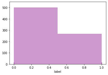
sns.distplot(data['label'], kde = False, rug= True, color ='purple', bins=2)
/opt/jupyterhub/lib/python3.8/site-packages/seaborn/distributions.py:2619: FutureWarning: `distplot` is a deprecated function and will be removed in a future version. Please adapt your code to use either `displot` (a figure-level function with similar flexibility) or `histplot` (an axes-level function for histograms).
  warnings.warn(msg, FutureWarning)
/opt/jupyterhub/lib/python3.8/site-packages/seaborn/distributions.py:2103: FutureWarning: The `axis` variable is no longer used and will be removed. Instead, assign variables directly to `x` or `y`.
  warnings.warn(msg, FutureWarning)
<AxesSubplot:xlabel='label'>
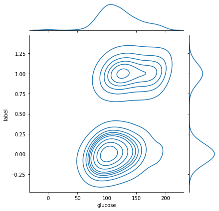
sns.jointplot(x ='glucose', y ='label', data = data, kind ='kde')
<seaborn.axisgrid.JointGrid at 0xffff51ab23a0>
Selecting Features:¶
Here, we need to divide the given columns into two types of variables dependent(or target variable) and independent variable(or feature variables or predictors).
#split dataset in features and target variable
feature_cols = ['pregnant', 'glucose', 'bp', 'skin', 'Insulin', 'bmi', 'pedigree', 'age']
X = data[feature_cols] # Features
y = data.label # Target variable
Splitting Data:¶
To understand model performance, dividing the dataset into a training set and a test set is a good strategy. Let’s split dataset by using function train_test_split(). You need to pass 3 parameters: features, target, and test_set size. Additionally, you can use random_state to select records randomly. Here, the Dataset is broken into two parts in a ratio of 75:25. It means 75% data will be used for model training and 25% for model testing:
# split X and y into training and testing sets
from sklearn.model_selection import train_test_split
X_train,X_test,y_train,y_test=train_test_split(X,y,test_size=0.25,random_state=0)
Model Development and Prediction:¶
First, import the Logistic Regression module and create a Logistic Regression classifier object using LogisticRegression() function. Then, fit your model on the train set using fit() and perform prediction on the test set using predict().
# import the class
from sklearn.linear_model import LogisticRegression

# instantiate the model (using the default parameters)
#logreg = LogisticRegression()
logreg = LogisticRegression()
# fit the model with data
logreg.fit(X_train,y_train)

#
y_pred=logreg.predict(X_test)
/opt/jupyterhub/lib/python3.8/site-packages/sklearn/linear_model/_logistic.py:814: ConvergenceWarning: lbfgs failed to converge (status=1):
STOP: TOTAL NO. of ITERATIONS REACHED LIMIT.

Increase the number of iterations (max_iter) or scale the data as shown in:
    https://scikit-learn.org/stable/modules/preprocessing.html
Please also refer to the documentation for alternative solver options:
    https://scikit-learn.org/stable/modules/linear_model.html#logistic-regression
  n_iter_i = _check_optimize_result(

How to assess the performance of logistic regression?
Binary classification has four possible types of results:
True negatives: correctly predicted negatives (zeros)
True positives: correctly predicted positives (ones)
False negatives: incorrectly predicted negatives (zeros)
False positives: incorrectly predicted positives (ones)
We usually evaluate the performance of a classifier by comparing the actual and predicted outputsand counting the correct and incorrect predictions. A confusion matrix is a table that is used to evaluate the performance of a classification model.
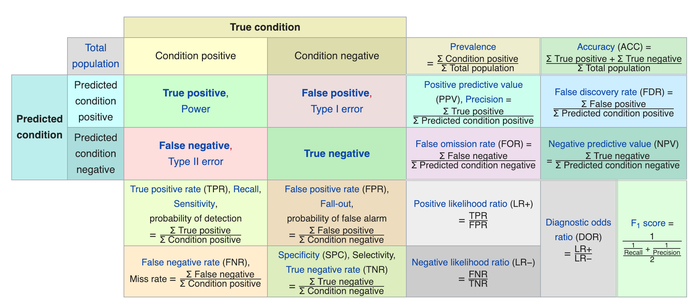
Some indicators of binary classifiers include the following:
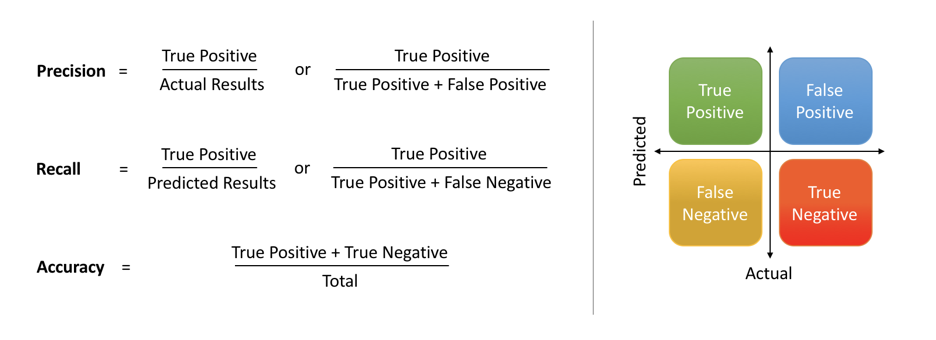
The most straightforward indicator of classification accuracy is the ratio of the number of correct predictions to the total number of predictions (or observations).
The positive predictive value is the ratio of the number of true positives to the sum of the numbers of true and false positives.
The negative predictive value is the ratio of the number of true negatives to the sum of the numbers of true and false negatives.
The sensitivity (also known as recall or true positive rate) is the ratio of the number of true positives to the number of actual positives.
The precision score quantifies the ability of a classifier to not label a negative example as positive. The precision score can be interpreted as the probability that a positive prediction made by the classifier is positive.
The specificity (or true negative rate) is the ratio of the number of true negatives to the number of actual negatives.
The extent of importance of recall and precision depends on the problem. Achieving a high recall is more important than getting a high precision in cases like when we would like to detect as many heart patients as possible. For some other models, like classifying whether a bank customer is a loan defaulter or not, it is desirable to have a high precision since the bank wouldn’t want to lose customers who were denied a loan based on the model’s prediction that they would be defaulters.
There are also a lot of situations where both precision and recall are equally important. Then we would aim for not only a high recall but a high precision as well. In such cases, we use something called F1-score. F1-score is the Harmonic mean of the Precision and Recall:
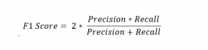
This is easier to work with since now, instead of balancing precision and recall, we can just aim for a good F1-score and that would be indicative of a good Precision and a good Recall value as well.

Model Evaluation using Confusion Matrix:¶
A confusion matrix is a table that is used to evaluate the performance of a classification model. You can also visualize the performance of an algorithm. The fundamental of a confusion matrix is the number of correct and incorrect predictions are summed up class-wise.
# import the metrics class
from sklearn import metrics
cnf_matrix = metrics.confusion_matrix(y_pred, y_test)
cnf_matrix
array([[115,  25],
       [ 15,  37]])
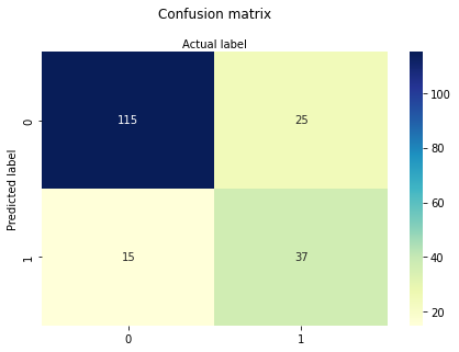
Here, you can see the confusion matrix in the form of the array object. The dimension of this matrix is 2*2 because this model is binary classification. You have two classes 0 and 1. Diagonal values represent accurate predictions, while non-diagonal elements are inaccurate predictions. In the output, 119 and 36 are actual predictions, and 26 and 11 are incorrect predictions.
Visualizing Confusion Matrix using Heatmap:¶
Let’s visualize the results of the model in the form of a confusion matrix using matplotlib and seaborn.
class_names=[0,1] # name  of classes
fig, ax = plt.subplots()
tick_marks = np.arange(len(class_names))
plt.xticks(tick_marks, class_names)
plt.yticks(tick_marks, class_names)
# create heatmap
sns.heatmap(pd.DataFrame(cnf_matrix), annot=True, cmap="YlGnBu" ,fmt='g')
ax.xaxis.set_label_position("top")
plt.tight_layout()
plt.title('Confusion matrix', y=1.1)
plt.ylabel('Predicted label')
plt.xlabel('Actual label')
Text(0.5, 257.44, 'Actual label')
Confusion Matrix Evaluation Metrics:¶
Let’s evaluate the model using model evaluation metrics such as accuracy, precision, and recall.
print("Accuracy:",metrics.accuracy_score(y_test, y_pred))
print("Precision:",metrics.precision_score(y_test, y_pred))
print("Recall:",metrics.recall_score(y_test, y_pred))
print("F1-score:",metrics.f1_score(y_test, y_pred))
Accuracy: 0.7916666666666666
Precision: 0.7115384615384616
Recall: 0.5967741935483871
F1-score: 0.6491228070175439
from sklearn.metrics import classification_report

print(classification_report(y_test, y_pred))
              precision    recall  f1-score   support

           0       0.82      0.88      0.85       130
           1       0.71      0.60      0.65        62

    accuracy                           0.79       192
   macro avg       0.77      0.74      0.75       192
weighted avg       0.79      0.79      0.79       192

Credit Card Fraud Detection
¶

For many companies, losses involving transaction fraud amount to more than 10% of their total expenses. The concern with these massive losses leads companies to constantly seek new solutions to prevent, detect and eliminate fraud. Machine Learning is one of the most promising technological weapons to combat financial fraud. The objective of this project is to create a simple Logistic Regression model capable of detecting fraud in credit card operations, thus seeking to minimize the risk and loss of the business.
The dataset used contains transactions carried out by European credit card holders that took place over two days in September 2013, and is a shorter version of a dataset that is available on kaggle at https://www.kaggle.com/mlg-ulb/creditcardfraud/version/3.
“It contains only numerical input variables which are the result of a PCA (Principal Component Analysis) transformation. Unfortunately, due to confidentiality issues, we cannot provide the original features and more background information about the data. Features V1, V2, … V28 are the principal components obtained with PCA, the only features which have not been transformed with PCA are ‘Time’ and ‘Amount’. Feature ‘Time’ contains the seconds elapsed between each transaction and the first transaction in the dataset. The feature ‘Amount’ is the transaction Amount, this feature can be used for example-dependant cost-senstive learning. Feature ‘Class’ is the response variable and it takes value 1 in case of fraud and 0 otherwise.”
Columns |
Info. |
|---|---|
Time |
Number of seconds elapsed between this transaction and the first transaction in the dataset |
V1-V28 |
Result of a PCA Dimensionality reduction to protect user identities and sensitive features(v1-v28) |
Amount |
Transaction amount |
Class |
1 for fraudulent transactions, 0 otherwise |
Note
Principal Component Analysis, or PCA, is a dimensionality-reduction method that is often used to reduce the dimensionality of large data sets, by transforming a large set of variables into a smaller one that still contains most of the information in the large set.
Acknowledgements The dataset has been collected and analysed during a research collaboration of Worldline and the Machine Learning Group (http://mlg.ulb.ac.be) of ULB (Université Libre de Bruxelles) on big data mining and fraud detection. More details on current and past projects on related topics are available on https://www.researchgate.net/project/Fraud-detection-5 and the page of the DefeatFraud project
Please cite the following works:
Andrea Dal Pozzolo, Olivier Caelen, Reid A. Johnson and Gianluca Bontempi. Calibrating Probability with Undersampling for Unbalanced Classification. In Symposium on Computational Intelligence and Data Mining (CIDM), IEEE, 2015
Dal Pozzolo, Andrea; Caelen, Olivier; Le Borgne, Yann-Ael; Waterschoot, Serge; Bontempi, Gianluca. Learned lessons in credit card fraud detection from a practitioner perspective, Expert systems with applications,41,10,4915-4928,2014, Pergamon
Dal Pozzolo, Andrea; Boracchi, Giacomo; Caelen, Olivier; Alippi, Cesare; Bontempi, Gianluca. Credit card fraud detection: a realistic modeling and a novel learning strategy, IEEE transactions on neural networks and learning systems,29,8,3784-3797,2018,IEEE
Dal Pozzolo, Andrea Adaptive Machine learning for credit card fraud detection ULB MLG PhD thesis (supervised by G. Bontempi)
Carcillo, Fabrizio; Dal Pozzolo, Andrea; Le Borgne, Yann-Aël; Caelen, Olivier; Mazzer, Yannis; Bontempi, Gianluca. Scarff: a scalable framework for streaming credit card fraud detection with Spark, Information fusion,41, 182-194,2018,Elsevier
Carcillo, Fabrizio; Le Borgne, Yann-Aël; Caelen, Olivier; Bontempi, Gianluca. Streaming active learning strategies for real-life credit card fraud detection: assessment and visualization, International Journal of Data Science and Analytics, 5,4,285-300,2018,Springer International Publishing
Bertrand Lebichot, Yann-Aël Le Borgne, Liyun He, Frederic Oblé, Gianluca Bontempi Deep-Learning Domain Adaptation Techniques for Credit Cards Fraud Detection, INNSBDDL 2019: Recent Advances in Big Data and Deep Learning, pp 78-88, 2019
Fabrizio Carcillo, Yann-Aël Le Borgne, Olivier Caelen, Frederic Oblé, Gianluca Bontempi Combining Unsupervised and Supervised Learning in Credit Card Fraud Detection Information Sciences, 2019
As you know by now, the first step is to load some necessary libraries:
import numpy as np
import pandas as pd
from matplotlib import pyplot as plt
import sklearn.metrics as metrics
import seaborn as sns
%matplotlib inline
Then, we should read the dataset and explore it using tools such as descriptive statistics:
# Import the dataset:
data = pd.read_csv("creditcard_m.csv")
data.head()
| Time | V1 | V2 | V3 | V4 | V5 | V6 | V7 | V8 | V9 | ... | V21 | V22 | V23 | V24 | V25 | V26 | V27 | V28 | Amount | Class | |
|---|---|---|---|---|---|---|---|---|---|---|---|---|---|---|---|---|---|---|---|---|---|
| 0 | 0 | -1.359807 | -0.072781 | 2.536347 | 1.378155 | -0.338321 | 0.462388 | 0.239599 | 0.098698 | 0.363787 | ... | -0.018307 | 0.277838 | -0.110474 | 0.066928 | 0.128539 | -0.189115 | 0.133558 | -0.021053 | 149.62 | 0 |
| 1 | 0 | 1.191857 | 0.266151 | 0.166480 | 0.448154 | 0.060018 | -0.082361 | -0.078803 | 0.085102 | -0.255425 | ... | -0.225775 | -0.638672 | 0.101288 | -0.339846 | 0.167170 | 0.125895 | -0.008983 | 0.014724 | 2.69 | 0 |
| 2 | 1 | -1.358354 | -1.340163 | 1.773209 | 0.379780 | -0.503198 | 1.800499 | 0.791461 | 0.247676 | -1.514654 | ... | 0.247998 | 0.771679 | 0.909412 | -0.689281 | -0.327642 | -0.139097 | -0.055353 | -0.059752 | 378.66 | 0 |
| 3 | 1 | -0.966272 | -0.185226 | 1.792993 | -0.863291 | -0.010309 | 1.247203 | 0.237609 | 0.377436 | -1.387024 | ... | -0.108300 | 0.005274 | -0.190321 | -1.175575 | 0.647376 | -0.221929 | 0.062723 | 0.061458 | 123.50 | 0 |
| 4 | 2 | -1.158233 | 0.877737 | 1.548718 | 0.403034 | -0.407193 | 0.095921 | 0.592941 | -0.270533 | 0.817739 | ... | -0.009431 | 0.798278 | -0.137458 | 0.141267 | -0.206010 | 0.502292 | 0.219422 | 0.215153 | 69.99 | 0 |
5 rows × 31 columns
As expected, the dataset has 31 columns and the target variable is located in the last one. Let’s check and see whether we have any missing values in the dataset:
data.isnull().sum()
Time      0
V1        0
V2        0
V3        0
V4        0
V5        0
V6        0
V7        0
V8        0
V9        0
V10       0
V11       0
V12       0
V13       0
V14       0
V15       0
V16       0
V17       0
V18       0
V19       0
V20       0
V21       0
V22       0
V23       0
V24       0
V25       0
V26       0
V27       0
V28       0
Amount    0
Class     0
dtype: int64
Great! No missing values!
data.describe()
| Time | V1 | V2 | V3 | V4 | V5 | V6 | V7 | V8 | V9 | ... | V21 | V22 | V23 | V24 | V25 | V26 | V27 | V28 | Amount | Class | |
|---|---|---|---|---|---|---|---|---|---|---|---|---|---|---|---|---|---|---|---|---|---|
| count | 140000.000000 | 140000.000000 | 140000.000000 | 140000.000000 | 140000.000000 | 140000.000000 | 140000.000000 | 140000.000000 | 140000.000000 | 140000.000000 | ... | 140000.000000 | 140000.000000 | 140000.000000 | 140000.000000 | 140000.000000 | 140000.000000 | 140000.000000 | 140000.000000 | 140000.000000 | 140000.000000 |
| mean | 51858.089636 | -0.249409 | 0.017429 | 0.672713 | 0.139812 | -0.282655 | 0.078898 | -0.117062 | 0.065205 | -0.092188 | ... | -0.039503 | -0.118547 | -0.033419 | 0.012095 | 0.130218 | 0.023580 | 0.000651 | 0.002244 | 91.210270 | 0.001886 |
| std | 20867.521978 | 1.816521 | 1.614340 | 1.268657 | 1.322410 | 1.307926 | 1.284004 | 1.166853 | 1.230046 | 1.088755 | ... | 0.721638 | 0.635371 | 0.591946 | 0.595760 | 0.437298 | 0.492026 | 0.389003 | 0.307370 | 247.334466 | 0.043384 |
| min | 0.000000 | -56.407510 | -72.715728 | -33.680984 | -5.519697 | -42.147898 | -26.160506 | -31.764946 | -73.216718 | -9.283925 | ... | -34.830382 | -10.933144 | -44.807735 | -2.836627 | -10.295397 | -2.534330 | -22.565679 | -11.710896 | 0.000000 | 0.000000 |
| 25% | 37912.750000 | -1.020760 | -0.564561 | 0.170073 | -0.714009 | -0.903653 | -0.662022 | -0.603820 | -0.131071 | -0.714753 | ... | -0.226206 | -0.548060 | -0.171763 | -0.324841 | -0.136182 | -0.326158 | -0.060305 | -0.004172 | 6.000000 | 0.000000 |
| 50% | 53665.500000 | -0.269833 | 0.104206 | 0.750038 | 0.167473 | -0.314849 | -0.176600 | -0.064160 | 0.080302 | -0.154499 | ... | -0.059815 | -0.095518 | -0.044999 | 0.068815 | 0.166593 | -0.064948 | 0.011781 | 0.023609 | 23.920000 | 0.000000 |
| 75% | 69322.000000 | 1.157985 | 0.776185 | 1.363041 | 0.993562 | 0.237514 | 0.465404 | 0.409714 | 0.374985 | 0.482352 | ... | 0.113587 | 0.301082 | 0.083271 | 0.408740 | 0.418787 | 0.287195 | 0.087053 | 0.077127 | 81.000000 | 0.000000 |
| max | 83479.000000 | 1.960497 | 18.902453 | 9.382558 | 16.715537 | 34.801666 | 22.529298 | 36.677268 | 20.007208 | 15.594995 | ... | 27.202839 | 10.503090 | 19.002942 | 4.022866 | 5.541598 | 3.517346 | 12.152401 | 33.847808 | 19656.530000 | 1.000000 |
8 rows × 31 columns
print ('Not Fraud % ',round(data['Class'].value_counts()[0]/len(data)*100,2))
print ()
print (round(data.Amount[data.Class == 0].describe(),2))
print ()
print ()
print ('Fraud %    ',round(data['Class'].value_counts()[1]/len(data)*100,2))
print ()
print (round(data.Amount[data.Class == 1].describe(),2))
Not Fraud %  99.81

count    139736.00
mean         91.16
std         247.34
min           0.00
25%           6.02
50%          23.94
75%          80.92
max       19656.53
Name: Amount, dtype: float64


Fraud %     0.19

count     264.00
mean      115.39
std       245.19
min         0.00
25%         1.00
50%         9.56
75%        99.99
max      1809.68
Name: Amount, dtype: float64
We have a total of 140000 samples in this dataset. The PCA components (V1-V28) look as if they have similar spreads and rather small mean values in comparison to another predictors such as ‘Time’. The majority (75%) of transactions are below 81 euros with some considerably high outliers (the max is 19656.53 euros). Around 0.19% of all the observed transactions were found to be fraudulent which means that we are dealing with an extremely unbalanced dataset. An important characteristic of such problems. Although the share may seem small, each fraud transaction can represent a very significant expense, which together can represent billions of dollars of lost revenue each year.
The next step is to define our predictors and target:
#split dataset in features and target variable
y = data.Class # Target variable
X = data.loc[:, data.columns != "Class"] # Features
The next step would be to split our dataset and define the training and testing sets. The random seed (np.random.seed) is used to ensure that the same data is used for all runs. Let’s do a 70/30 split:
# split X and y into training and testing sets
np.random.seed(123)

from sklearn.model_selection import train_test_split
X_train,X_test,y_train,y_test=train_test_split(X,y,test_size=0.30,random_state=1)
Now it is time for model development and prediction!
import the Logistic Regression module and create a Logistic Regression classifier object using LogisticRegression() function. Then, fit your model on the train set using fit() and perform prediction on the test set using predict().
# import the class
from sklearn.linear_model import LogisticRegression

# instantiate the model (using the default parameters)
#logreg = LogisticRegression()
logreg = LogisticRegression(solver='lbfgs',max_iter=10000)
# fit the model with data  -TRAIN the model
logreg.fit(X_train,y_train)
LogisticRegression(max_iter=10000)
# TEST the model
y_pred=logreg.predict(X_test)
Once the model and the predictions are ready, we can assess the performance of our classifier. First, we need to get our confusion matrix:
A confusion matrix is a table that is used to evaluate the performance of a classification model. You can also visualize the performance of an algorithm. The fundamental of a confusion matrix is the number of correct and incorrect predictions are summed up class-wise.
from sklearn import metrics
cnf_matrix = metrics.confusion_matrix(y_pred, y_test)
print(cnf_matrix)
tpos = cnf_matrix[0][0]
fneg = cnf_matrix[1][1]
fpos = cnf_matrix[0][1]
tneg = cnf_matrix[1][0]
print("True Positive Cases are",tpos) #How many non-fraud cases were identified as non-fraud cases - GOOD
print("True Negative Cases are",tneg) #How many Fraud cases were identified as Fraud cases - GOOD
print("False Positive Cases are",fpos) #How many Fraud cases were identified as non-fraud cases - BAD | (type 1 error)
print("False Negative Cases are",fneg) #How many non-fraud cases were identified as Fraud cases - BAD | (type 2 error)
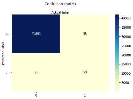
[[41891    38]
 [   21    50]]
True Positive Cases are 41891
True Negative Cases are 21
False Positive Cases are 38
False Negative Cases are 50
class_names=[0,1] # name  of classes
fig, ax = plt.subplots()
tick_marks = np.arange(len(class_names))
plt.xticks(tick_marks, class_names)
plt.yticks(tick_marks, class_names)
# create heatmap
sns.heatmap(pd.DataFrame(cnf_matrix), annot=True, cmap="YlGnBu" ,fmt='g')
ax.xaxis.set_label_position("top")
plt.tight_layout()
plt.title('Confusion matrix', y=1.1)
plt.ylabel('Predicted label')
plt.xlabel('Actual label')
Text(0.5, 257.44, 'Actual label')
We should go further and evaluate the model using model evaluation metrics such as accuracy, precision, and recall. These are calculated based on the confustion matrix:
print("Accuracy:",metrics.accuracy_score(y_test, y_pred))
Accuracy: 0.9985952380952381
That is a fantastic accuracy score, isn’t it?
print("Precision:",metrics.precision_score(y_test, y_pred))
print("Recall:",metrics.recall_score(y_test, y_pred))
print("F1-score:",metrics.f1_score(y_test, y_pred))
Precision: 0.704225352112676
Recall: 0.5681818181818182
F1-score: 0.6289308176100629
from sklearn.metrics import classification_report

print(classification_report(y_test, y_pred))
              precision    recall  f1-score   support

           0       1.00      1.00      1.00     41912
           1       0.70      0.57      0.63        88

    accuracy                           1.00     42000
   macro avg       0.85      0.78      0.81     42000
weighted avg       1.00      1.00      1.00     42000
Although the accuracy is excellent, the model struggles with fraud detection and has not captured about 30 out of 71 fraudulent transactions.
Accuracy in a highly unbalanced data set does not represent a correct value for the efficiency of a model. That’s where precision, recall and more specifically F1-score as their combinations becomes important:
Accuracy is used when the True Positives and True negatives are more important while F1-score is used when the False Negatives and False Positives are crucial
Accuracy can be used when the class distribution is similar while F1-score is a better metric when there are imbalanced classes as in the above case.
In most real-life classification problems, imbalanced class distribution exists and thus F1-score is a better metric to evaluate our model on.

This notebook was inspired by several blogposts including:
“Logistic Regression in Python” by Mirko Stojiljković available at* https://realpython.com/logistic-regression-python/
“Understanding Logistic Regression in Python” by Avinash Navlani available at* https://www.datacamp.com/community/tutorials/understanding-logistic-regression-python
“Understanding Logistic Regression with Python: Practical Guide 1” by Mayank Tripathi available at* https://datascience.foundation/sciencewhitepaper/understanding-logistic-regression-with-python-practical-guide-1
“Understanding Data Science Classification Metrics in Scikit-Learn in Python” by Andrew Long available at* https://towardsdatascience.com/understanding-data-science-classification-metrics-in-scikit-learn-in-python-3bc336865019
Here are some great reads on these topics:
“Example of Logistic Regression in Python” available at* https://datatofish.com/logistic-regression-python/
“Building A Logistic Regression in Python, Step by Step” by Susan Li available at* https://towardsdatascience.com/building-a-logistic-regression-in-python-step-by-step-becd4d56c9c8
“How To Perform Logistic Regression In Python?” by Mohammad Waseem available at* https://www.edureka.co/blog/logistic-regression-in-python/
“Logistic Regression in Python Using Scikit-learn” by Dhiraj K available at* https://heartbeat.fritz.ai/logistic-regression-in-python-using-scikit-learn-d34e882eebb1
“ML | Logistic Regression using Python” available at* https://www.geeksforgeeks.org/ml-logistic-regression-using-python/
Here are some great videos on these topics:
“StatQuest: Logistic Regression” by StatQuest with Josh Starmer available at* https://www.youtube.com/watch?v=yIYKR4sgzI8&list=PLblh5JKOoLUKxzEP5HA2d-Li7IJkHfXSe
“Linear Regression vs Logistic Regression | Data Science Training | Edureka” by edureka! available at* https://www.youtube.com/watch?v=OCwZyYH14uw
“Logistic Regression in Python | Logistic Regression Example | Machine Learning Algorithms | Edureka” by edureka! available at* https://www.youtube.com/watch?v=VCJdg7YBbAQ
“How to evaluate a classifier in scikit-learn” by Data School available at* https://www.youtube.com/watch?v=85dtiMz9tSo
“How to evaluate a classifier in scikit-learn” by Data School available at* https://www.youtube.com/watch?v=85dtiMz9tSo

Exercise: Logistic Regression in Engineering
¶
topic¶
From Wikipedia (https://en.wikipedia.org/wiki/Logistic_regression) (emphasis is mine):
In statistics, the logistic model (or logit model) is used to model the probability of a certain class or event existing such as pass/fail, win/lose, alive/dead or healthy/sick. This can be extended to model several classes of events such as determining whether an image contains a cat, dog, lion, etc. Each object being detected in the image would be assigned a probability between 0 and 1, with a sum of one.
Logistic regression is a statistical model that in its basic form uses a logistic function to model a binary dependent variable, although many more complex extensions exist. In regression analysis, logistic regression (or logit regression) is estimating the parameters of a logistic model (a form of binary regression). Mathematically, a binary logistic model has a dependent variable with two possible values, such as pass/fail which is represented by an indicator variable, where the two values are labeled “0” and “1”. In the logistic model, the log-odds (the logarithm of the odds) for the value labeled “1” is a linear combination of one or more independent variables (“predictors”); the independent variables can each be a binary variable (two classes, coded by an indicator variable) or a continuous variable (any real value).
The corresponding probability of the value labeled “1” can vary between 0 (certainly the value “0”) and 1 (certainly the value “1”), hence the labeling; the function that converts log-odds to probability is the logistic function, hence the name. The unit of measurement for the log-odds scale is called a logit, from logistic unit, hence the alternative names. Analogous models with a different sigmoid function instead of the logistic function can also be used, such as the probit model; the defining characteristic of the logistic model is that increasing one of the independent variables multiplicatively scales the odds of the given outcome at a constant rate, with each independent variable having its own parameter; for a binary dependent variable this generalizes the odds ratio.
In a binary logistic regression model, the dependent variable has two levels (categorical). Outputs with more than two values are modeled by multinomial logistic regression and, if the multiple categories are ordered, by ordinal logistic regression (for example the proportional odds ordinal logistic model). The logistic regression model itself simply models probability of output in terms of input and does not perform statistical classification (it is not a classifier), though it can be used to make a classifier, for instance by choosing a cutoff value and classifying inputs with probability greater than the cutoff as one class, below the cutoff as the other; this is a common way to make a binary classifier. The coefficients are generally not computed by a closed-form expression, unlike linear least squares; see § Model fitting. \(\dots\)
Now lets visit the Wiki and learn more https://en.wikipedia.org/wiki/Logistic_regression
Now lets visit our friends at towardsdatascience https://towardsdatascience.com/logistic-regression-detailed-overview-46c4da4303bc Here we will literally CCMR the scripts there.
We need the data, a little searching and its here https://gist.github.com/curran/a08a1080b88344b0c8a7 after download and extract we will need to rename the database
lorem ipsum
import numpy as np
import pandas as pd
import matplotlib.pyplot as plt
%matplotlib inline
import seaborn as sns
import sklearn
from sklearn.model_selection import train_test_split
from sklearn.preprocessing import StandardScaler
from sklearn.metrics import accuracy_score
df = pd.read_csv('iris-data.csv')
df.head()
| sepal_length_cm | sepal_width_cm | petal_length_cm | petal_width_cm | class | |
|---|---|---|---|---|---|
| 0 | 5.1 | 3.5 | 1.4 | 0.2 | Iris-setosa |
| 1 | 4.9 | 3.0 | 1.4 | 0.2 | Iris-setosa |
| 2 | 4.7 | 3.2 | 1.3 | 0.2 | Iris-setosa |
| 3 | 4.6 | 3.1 | 1.5 | 0.2 | Iris-setosa |
| 4 | 5.0 | 3.6 | 1.4 | 0.2 | Iris-setosa |
df.describe()
| sepal_length_cm | sepal_width_cm | petal_length_cm | petal_width_cm | |
|---|---|---|---|---|
| count | 150.000000 | 150.000000 | 150.000000 | 145.000000 |
| mean | 5.644627 | 3.054667 | 3.758667 | 1.236552 |
| std | 1.312781 | 0.433123 | 1.764420 | 0.755058 |
| min | 0.055000 | 2.000000 | 1.000000 | 0.100000 |
| 25% | 5.100000 | 2.800000 | 1.600000 | 0.400000 |
| 50% | 5.700000 | 3.000000 | 4.350000 | 1.300000 |
| 75% | 6.400000 | 3.300000 | 5.100000 | 1.800000 |
| max | 7.900000 | 4.400000 | 6.900000 | 2.500000 |
df.info()
<class 'pandas.core.frame.DataFrame'>
RangeIndex: 150 entries, 0 to 149
Data columns (total 5 columns):
 #   Column           Non-Null Count  Dtype
---  ------           --------------  -----
 0   sepal_length_cm  150 non-null    float64
 1   sepal_width_cm   150 non-null    float64
 2   petal_length_cm  150 non-null    float64
 3   petal_width_cm   145 non-null    float64
 4   class            150 non-null    object
dtypes: float64(4), object(1)
memory usage: 6.0+ KB
#Removing all null values row
df = df.dropna(subset=['petal_width_cm'])
df.info()
<class 'pandas.core.frame.DataFrame'>
Int64Index: 145 entries, 0 to 149
Data columns (total 5 columns):
 #   Column           Non-Null Count  Dtype
---  ------           --------------  -----
 0   sepal_length_cm  145 non-null    float64
 1   sepal_width_cm   145 non-null    float64
 2   petal_length_cm  145 non-null    float64
 3   petal_width_cm   145 non-null    float64
 4   class            145 non-null    object
dtypes: float64(4), object(1)
memory usage: 6.8+ KB
#Plot
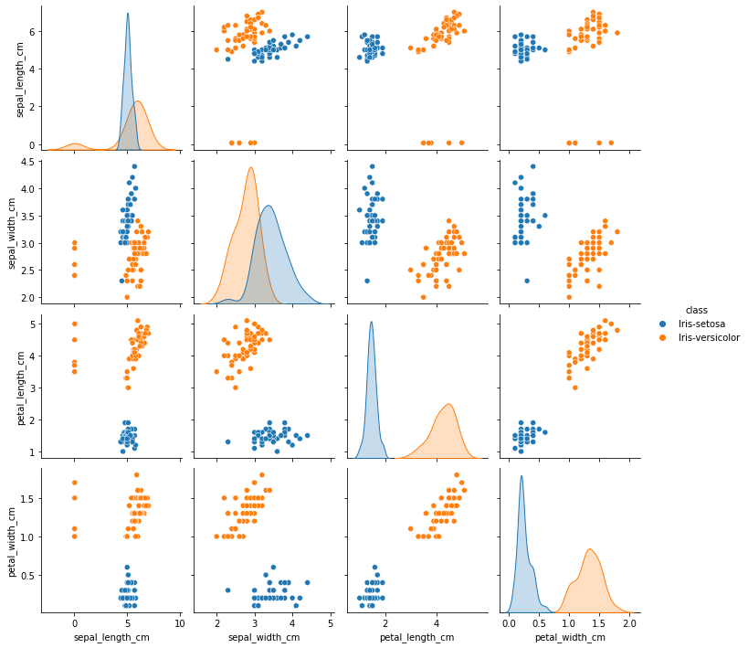
sns.pairplot(df, hue='class', height=2.5)
<seaborn.axisgrid.PairGrid at 0xffff53eb4d30>
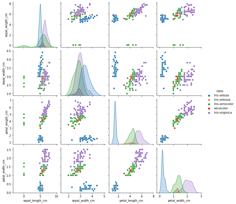
From the plots it can be observed that there is some abnormality in the class name. Let’s explore further
df['class'].value_counts()
Iris-virginica     50
Iris-versicolor    45
Iris-setosa        44
versicolor          5
Iris-setossa        1
Name: class, dtype: int64
Two observations can be made from the above results
For 5 data points ‘Iris-versicolor’ has been specified as ‘versicolor’
For 1 data points, ‘Iris-setosa’ has been specified as ‘Iris-setossa’
df['class'].replace(["Iris-setossa","versicolor"], ["Iris-setosa","Iris-versicolor"], inplace=True)
df['class'].value_counts()
Iris-versicolor    50
Iris-virginica     50
Iris-setosa        45
Name: class, dtype: int64
Simple Logistic Regression¶
Consider only two class ‘Iris-setosa’ and ‘Iris-versicolor’. Dropping all other class
final_df = df[df['class'] != 'Iris-virginica']
final_df.head()
| sepal_length_cm | sepal_width_cm | petal_length_cm | petal_width_cm | class | |
|---|---|---|---|---|---|
| 0 | 5.1 | 3.5 | 1.4 | 0.2 | Iris-setosa |
| 1 | 4.9 | 3.0 | 1.4 | 0.2 | Iris-setosa |
| 2 | 4.7 | 3.2 | 1.3 | 0.2 | Iris-setosa |
| 3 | 4.6 | 3.1 | 1.5 | 0.2 | Iris-setosa |
| 4 | 5.0 | 3.6 | 1.4 | 0.2 | Iris-setosa |
Outlier Check¶
sns.pairplot(final_df, hue='class', height=2.5)
<seaborn.axisgrid.PairGrid at 0xffff4b4cb340>
From the above plot, sepal_width and sepal_length seems to have outliers. To confirm let’s plot them seperately
SEPAL LENGTH
final_df.hist(column = 'sepal_length_cm',bins=20, figsize=(10,5))
array([[<AxesSubplot:title={'center':'sepal_length_cm'}>]], dtype=object)
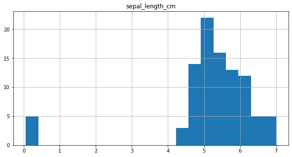
It can be observed from the plot, that for 5 data points values are below 1 and they seem to be outliers. So, these data points are considered to be in ‘m’ and are converted to ‘cm’.
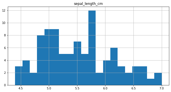
final_df.loc[final_df.sepal_length_cm < 1, ['sepal_length_cm']] = final_df['sepal_length_cm']*100
final_df.hist(column = 'sepal_length_cm',bins=20, figsize=(10,5))
/opt/jupyterhub/lib/python3.8/site-packages/pandas/core/indexing.py:1734: SettingWithCopyWarning:
A value is trying to be set on a copy of a slice from a DataFrame.
Try using .loc[row_indexer,col_indexer] = value instead

See the caveats in the documentation: https://pandas.pydata.org/pandas-docs/stable/user_guide/indexing.html#returning-a-view-versus-a-copy
  isetter(loc, value[:, i].tolist())
array([[<AxesSubplot:title={'center':'sepal_length_cm'}>]], dtype=object)
SEPAL WIDTH
final_df = final_df.drop(final_df[(final_df['class'] == "Iris-setosa") & (final_df['sepal_width_cm'] < 2.5)].index)
sns.pairplot(final_df, hue='class', height=2.5)
<seaborn.axisgrid.PairGrid at 0xffff4ad35f70>
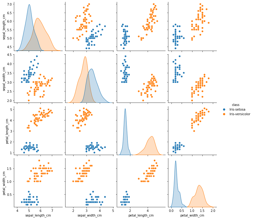
Successfully removed outliers!!
Label Encoding¶
final_df['class'].replace(["Iris-setosa","Iris-versicolor"], [1,0], inplace=True)
final_df.head()
| sepal_length_cm | sepal_width_cm | petal_length_cm | petal_width_cm | class | |
|---|---|---|---|---|---|
| 0 | 5.1 | 3.5 | 1.4 | 0.2 | 1 |
| 1 | 4.9 | 3.0 | 1.4 | 0.2 | 1 |
| 2 | 4.7 | 3.2 | 1.3 | 0.2 | 1 |
| 3 | 4.6 | 3.1 | 1.5 | 0.2 | 1 |
| 4 | 5.0 | 3.6 | 1.4 | 0.2 | 1 |
Model Construction¶
inp_df = final_df.drop(final_df.columns[[4]], axis=1)
out_df = final_df.drop(final_df.columns[[0,1,2,3]], axis=1)
#
scaler = StandardScaler()
inp_df = scaler.fit_transform(inp_df)
#
X_train, X_test, y_train, y_test = train_test_split(inp_df, out_df, test_size=0.2, random_state=42)
X_tr_arr = X_train
X_ts_arr = X_test
#y_tr_arr = y_train.as_matrix() # method deprecated several versions ago
#y_ts_arr = y_test.as_matrix()
y_tr_arr = y_train.values
y_ts_arr = y_test.values
print('Input Shape', (X_tr_arr.shape))
print('Output Shape', X_test.shape)
Input Shape (75, 4)
Output Shape (19, 4)
def weightInitialization(n_features):
    w = np.zeros((1,n_features))
    b = 0
    return w,b
def sigmoid_activation(result):
    final_result = 1/(1+np.exp(-result))
    return final_result
def model_optimize(w, b, X, Y):
    m = X.shape[0]

    #Prediction
    final_result = sigmoid_activation(np.dot(w,X.T)+b)
    Y_T = Y.T
    cost = (-1/m)*(np.sum((Y_T*np.log(final_result)) + ((1-Y_T)*(np.log(1-final_result)))))
    #

    #Gradient calculation
    dw = (1/m)*(np.dot(X.T, (final_result-Y.T).T))
    db = (1/m)*(np.sum(final_result-Y.T))

    grads = {"dw": dw, "db": db}

    return grads, cost
def model_predict(w, b, X, Y, learning_rate, no_iterations):
    costs = []
    for i in range(no_iterations):
        #
        grads, cost = model_optimize(w,b,X,Y)
        #
        dw = grads["dw"]
        db = grads["db"]
        #weight update
        w = w - (learning_rate * (dw.T))
        b = b - (learning_rate * db)
        #

        if (i % 100 == 0):
            costs.append(cost)
            #print("Cost after %i iteration is %f" %(i, cost))

    #final parameters
    coeff = {"w": w, "b": b}
    gradient = {"dw": dw, "db": db}

    return coeff, gradient, costs
def predict(final_pred, m):
    y_pred = np.zeros((1,m))
    for i in range(final_pred.shape[1]):
        if final_pred[0][i] > 0.5:
            y_pred[0][i] = 1
    return y_pred
#Get number of features
n_features = X_tr_arr.shape[1]
print('Number of Features', n_features)
w, b = weightInitialization(n_features)
#Gradient Descent
coeff, gradient, costs = model_predict(w, b, X_tr_arr, y_tr_arr, learning_rate=0.0001,no_iterations=4500)
#Final prediction
w = coeff["w"]
b = coeff["b"]
print('Optimized weights', w)
print('Optimized intercept',b)
#
final_train_pred = sigmoid_activation(np.dot(w,X_tr_arr.T)+b)
final_test_pred = sigmoid_activation(np.dot(w,X_ts_arr.T)+b)
#
m_tr =  X_tr_arr.shape[0]
m_ts =  X_ts_arr.shape[0]
#
y_tr_pred = predict(final_train_pred, m_tr)
print('Training Accuracy',accuracy_score(y_tr_pred.T, y_tr_arr))
#
y_ts_pred = predict(final_test_pred, m_ts)
print('Test Accuracy',accuracy_score(y_ts_pred.T, y_ts_arr))
Number of Features 4
Optimized weights [[-0.13397714  0.13130132 -0.18248682 -0.18319564]]
Optimized intercept -0.024134631921343585
Training Accuracy 1.0
Test Accuracy 1.0
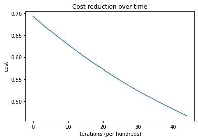
plt.plot(costs)
plt.ylabel('cost')
plt.xlabel('iterations (per hundreds)')
plt.title('Cost reduction over time')
plt.show()
from sklearn.linear_model import LogisticRegression
clf = LogisticRegression()
clf.fit(X_tr_arr, y_tr_arr)
/opt/jupyterhub/lib/python3.8/site-packages/sklearn/utils/validation.py:985: DataConversionWarning: A column-vector y was passed when a 1d array was expected. Please change the shape of y to (n_samples, ), for example using ravel().
  y = column_or_1d(y, warn=True)
LogisticRegression()
print (clf.intercept_, clf.coef_)
[-0.55607279] [[-0.69791666 1.16455265 -1.40231641 -1.47095115]]
pred = clf.predict(X_ts_arr)
print ('Accuracy from sk-learn: {0}'.format(clf.score(X_ts_arr, y_ts_arr)))
Accuracy from sk-learn: 1.0
References¶
Chan, Jamie. Machine Learning With Python For Beginners: A Step-By-Step Guide with Hands-On Projects (Learn Coding Fast with Hands-On Project Book 7) (p. 2). Kindle Edition.