
Common Data Types
Two “kinds” of data that exist are:
Quantitative
Qualitative
Quantitative Data
Quantitative data deals with numbers and refers to variables that can be mea- sured objectively. The root of the word is “quantity” which is an expression of how much of something exists.
The load on a building, the width of a channel, the temperature of lake, and the bearing capacity of a soil are quantitative data. While the meaning of the quantitative data is clear and unambigious there is uncertainty associated with them from measurement errors, transcription errors, and related causes.
Qualitative Data
Qualitative data refers descriptors that are subjective in nature. The root of the work is “quality” which is an expression of how desirable is the object.
Descriptors such as small loads, wide channel, sharp turn and extreme drought are some examples of qualitative data. The subjectivity arises because what is a small load for a large structure can be a substantial load for a small structure. The meaning of the qualitative data largely depends upon the situation and its interpretation can vary widely from one person to the next. Qualitative variables sometimes can be made quantitative for analysis. For example, flood is a qualitative variable. However, we can define a threshold flowrate to determine the flooding and non-flooding states in a river section.
Scale
Four common measurement scales of data are:
nominal,
ordinal,
interval, and
ratio scales.
Nominal Scale
The nominal scale is the simplest of all data scales. These data are qualitative and often used to label the data. For example, a traffic survey could ask a respondent’s gender (i.e., whether they are ’Male’ or ’Female’). The category ’Gender’ has two labels (Male and Female) which can be be used to filter data for further analysis. Nominal scale data have no order or hierarchy associated with them.
Ordinal Scale
The ordinal scale involves arranging data in an order. This ordering can be used to rank or compare two or more values. Ordinal scale also refers to qualitative data. For example we could classify droughts as ’mild’, moderate’ and ’severe’. Clearly severe droughts have far greater impacts than moderate droughts which in turn have a greater impact than mild droughts. We can also assign numeric values (say, 1 for mild, 2 for moderate and 3 for se- vere) to rank drought events in a region. However, we cannot do any arithmetic on these data (mild + moderate 6 = severe). Similarly the difference between a mild and moderate drought is not the same as the difference between a moderate and severe drought. Ordinal scales are often used to assess relative perceptions, choices and feedback.
Interval Scale
Interval scale data have an order and it is possible to calculate exact differences between the values. The interval scale is used with quantitative data. You can calculate summary measures (e.g., mean, variance) on interval scale data. The temperature measured in Celsius is a classic example of interval scale data. 20 oC is twice the value of 10 oC (i.e., the difference is 10 oC). Similarly, the difference between 90 oC and 80 oC is also 10 oC. This is because the values are being measured on the same interval. However, 20 oC is not twice as hot as 10 oC. This is evident when these temperatures are converted to the Fahrenheit scale (10 oC = 50 oF and 20 oC = 68 oF ). The reason for this is that there is no absolute zero in either Celsius of Fahrenheit scales. Zero just another measurement.
Ratio Scale
Variables measured on the ratio scale have an order, there are measured on fixed intervals (differences between two values can be calculated) and have an absolute zero. In other words, Ratio Scale has all the properties of an interval scale and also has an absolute zero. Ratio scale is used for quantitative data. Consider daily rainfall amounts. There is an absolute zero which corresponds to no rainfall. Other measurable amounts of rainfall are measured with respect to this absolute zero. 20’ of rainfall is more than 10’ of rainfall. Also, 20’ of rainfall is twice the amount of 10’ accumulation. Their ratio is equal to 2. In a similar vein, 3’ of rainfall is twice the amount of 6’ accumulation (again the ratio is 2). As the name suggests, variables measured on ratio scale can be divided to obtain ratios or the degree of proportionality between two observations. 3
Continuous and Discrete Data
Quantitative data can be further split into continuous and discrete data. Discrete data are integers and refer to variables that measure whole or indivisible entities. The number of vehicles passing an intersection over a year is discrete data as this is a whole number (integer).
Continuous data on the other hand are not restricted to integer values but also can take on fractional or decimal values. For example, The temperature of water in a lake can be 67.3\(^o\)F . Sometimes a variable that is continuous can be discretely measured or made discrete. For example, if we measure (or round off) the temperature of a lake to the nearest degree then we would have temperature measurements that are only integers. While continuous variables can be treated as discrete due to measurement limitations or data approximations, it is important to remember that intrinsically they can take continuous values and the discretization was simply a matter of convenience or a measurement limitation.
Summary measures of discrete variables (e.g., mean, standard deviation) can sometime have decimal values. For example, if 3 cars pass an intersection in the first hour and 4 cars in the second then the average number of cars is 3.5. In such instances, the value must be rounded appropriately (say to 4 if we are using it to estimate design loads on the pavement) as the decimal number is not physically realistic.
Continuous on a real line
Some variables in civil engineering are continuous on a real line (axis). For example, soil temperature measured in Celsius or Fahrenheit can assume both positive and negative values in cold regions. Similarly, the groundwater table measured with respect to mean sea level (MSL) can be either positive (i.e., below MSL) or negative (above MSL). A zero value simply suggests that the water table coincides with MSL which is just as a valid state as water table being above or below MSL. For variables that are continuous on a real line (axis), zero values have no special meaning and represent yet another value that the variable can take. In other words, they are often measured on an interval scale.
Positive Continuous Variables
As discussed above, the magnitude of a force is always positive. As this magni- tude can take decimal values it is a positive continuous variable. Many variables of interest to civil engineers are positive continuous. Flowrates, pollutant con- centrations, the magnitude of shear stresses are all positive continuous. Some variables that are continuous on a real line can also be made positive con- tinuous by shifting the datum. For example, there are no negative temperatures on Kelvin scale. Temperatures measured using Celsius scale can be made all positive by converting them into Kelvin scale. In a similar vein, the groundwa- ter table measurements at a well can be made all positive by measuring values from the top of the well casing (assuming positive downwards) instead of the mean sea level.
Mixture Datasets
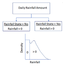
The positive continuous scale starts at zero and in theory extends all the way to infinity. For some positive continuous variables zero is yet another value if they are measured on the interval scale. On the other hand if they are measured on a ratio scale the value of zero is absolute and can assume special importance. For example, zero rainfall implies no rainfall. Therefore, a time-series data of daily rainfall in a year can have several values of zero (no rainfall) and some days with positive (non-zero rainfall). Such a dataset can be viewed as a mixture
At a high level the data is discrete where each day belongs to either (rain- fall=Yes) or (rainfall=No) state. Non-zero, positive continuous values exist for (Rainfall=Yes) state (see Figure 1).
Similar mixtures can also be seen with strictly discrete data. For example, if one were to count number of vehicles passing an intersection every hour of a day, there could be hours with no vehicles passing the intersection (traffic = No) and hours where some vehicles passed the intersection (traffic = Yes). A discrete dataset with non-zero values would correspond to the (traffic = Yes) state. It is therefore important to ascertain upfront whether the value of zero is a valid measurement for the questions we seek to address and how zero values will be handled during the analysis. Inclusion of a large number of zeros (zero- inflated datasets) will lower the mean and will affect other summary measures, on the other hand, exclusion of zero when it is a valid system response will lead to selection bias. The choices on how to handle zeros will depend upon the questions one seek to answer. It is important that the decision is made explicit and justified.
Truncated Data
Truncated data arise when values beyond a certain boundary are either not collected or removed prior to analysis. For example, the exclusion of zero values from a mixture data is one form of truncation.
Weigh-in-Motion (WIM) devices measure axle weights and gross vehicle weights of trucks while in motion. WIM data are used to estimate potential loads on bridges and also to select vehicles for static inspection (yep, profiling!). Trucks weighing below a certain weight are allowed to pass through or even when their weights are collected, the data is discarded when ascertaining design loads. There is a threshold load boundary that is used to truncate the data.
Flooding risks are often estimated using peak annual maximum flow data.
While flowrates are measured at a much higher rate (every 1 - 15 minutes), much of these data are discarded when assessing flooding risks. There is a threshold boundary that separates the maximum observed flow (state == max.flow) from the rest of the dataset (state != max. flow). However, the boundary in this case is not stable and varies annually. For example, The maximum flow obtained in a dry year could be lower than say the tenth highest flow observed in a wet year.
Truncation of data is also common when conducting or analyzing surveys . Certain surveys may target a specific age-group (teenage drivers) while exclud- ing others. Survey’s focused on environmental justice issues tend to focus on low-income neighborhoods in industrial areas. These data subsets are often extracted from larger ”quality of life” surveys that include respondents from different socioeconomic strata.
Truncation of data creates a selection bias; hence any truncation/censoring made explicitly during data analysis or implicitly during data collection must be well documented. Inferences drawn from the censored data will be biased towards the sub-population that was sampled and will not be representative of the entire population.
In a lot of applications truncating is appropriate, necessary, and understood - in instances where this is not so, disclosure is vital.
Censored Data
Censoring occurs when certain values in the dataset are only partially known. For example, a survey instrument measuring driving habits may classify the age group as ≤ 19 years. In this case, we know whether the respondent is below 20 years of age but we don’t know the exact age of each respondent.
Censoring also arises from instrument measurement limitations. Many instruments produce a small response even when there is no stimulus on the system. This response is referred to as the noise. The detection limit (DL) of an instrument is the lowest possible measurement that an instrument can make. This corresponds to a signal produced by the instrument that is significantly greater than the noise. When an instrument reports a value below its detection limit we cannot be fully confident of the value as the signal is affected by the noise. It is common to report such values as ≤ DL.
Let us say, a flowmeter can reliably measure flows that are at least 2 cfs. A censored dataset would arise if some of the measurements are below 2 cfs. A censored dataset would look like:
Measurement_ID |
Reported_Value |
|---|---|
808001 |
2.4 |
808002 |
3.2 |
808003 |
≤ 2.0 |
808004 |
2.1 |
808005 |
≤ 2.0 |
808006 |
2.3 |
\(\vdots\) |
\(\vdots\) |
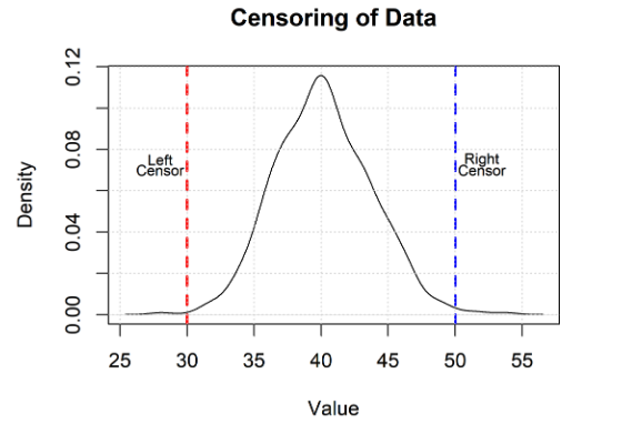
Censored data is a form of mixture data where some numbers are known with greater certainty and reported as numbers and others are known with less certainty and reported as inequalities. Left censoring refers to the situation where values below a threshold are not known with certainty and represented as inequalities. Instruments are designed to work correctly up to some specified upper limit. For example, a weighing scale may be designed to measure a maximum mass of 1000 kg. If we were to place a mass of 1200 kg on such a machine, we could ascertain that the mass is ≥ 1000 kg (instrument upper limit) but would not get a reading of 1200 kg. The dial on an analog scale would go past the maximum value of 1000 kg or a digital readout would raise an exception message stating the mass is over the instrument maximum limit. Situations where values above a threshold are uncertain are referred to as right censored data.
As another example, a traffic survey might categorize people over ≥ 70 years as elderly. Respondents who select these category are at least 75 years of age but we would not know how old they actually are.
It is not hard to conceive of situations where a dataset can be censored on both ends (i.e., be left and right censored). Such datasets are referred to as interval censored data
The figure below depicts the left and right censoring idea. The censoring occurs at values equal to 30 and 50. While the instrument may read a value of 25 or 55, because of the censoring they should be reported as ≤ 30 and ≥ 50 respectively.
Censoring versus Truncation
Censoring and truncation are distinct and should not be confused for one an- other. Both censoring and truncation define boundaries in the dataset. However, in censoring, we may be making (or have) measurements outside the boundaries. We don’t want to throw away or exclude the data that are outside the censoring boundaries. These are valid measurements but we don’t know their true values are.
On the other hand, in truncation, we are either not making measurements out- side the boundaries or willingly excluding data that are collected outside the truncation boundaries. Both truncation and censoring are distinct from round- ing where data are displayed to a specified number of significant digits to be consistent with the precision of the instrument and physical meaning of the variable.
Image Data
Images are usually arrays of signed integers or floats, that are interpreted by our programs to render what we see as an image. Underneath they are truncated data (black and white are used as upper and lower bounds depending on the color palette). Later on we will use image data and it will be important to have some feel for the underlying data.
Recall our cat image

Lets see it in gray scale
import numpy              # useful numerical routines
import scipy.special      # special functions library
import scipy.misc         # image processing code
import imageio            # image processing library
import matplotlib.pyplot  # import plotting routines
import warnings           # suppress warnings
warnings.filterwarnings('ignore')
img_array = imageio.imread("cat784.png", as_gray = True)
img_data1 = 255.0 - img_array.reshape(784)
img_data1 = ((img_data1/255.0)*0.99) + 0.01
matplotlib.pyplot.imshow(numpy.asfarray(img_data1).reshape((28,28)),cmap = 'Greys') # construct a graphic object #
matplotlib.pyplot.show() # show the graphic object to a window #
matplotlib.pyplot.close('all')
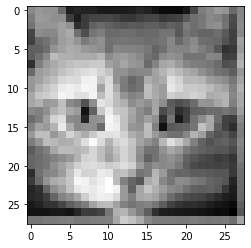
Now lets examine the 28x28 array of numbers that are representing our image
cat_data = numpy.asfarray(img_data1).reshape((28,28)) # extract image as 32-bit float
for irow in range(28):
    for jcol in range(28):
        cat_data[irow][jcol]=round(cat_data[irow][jcol],2) # round to 2 digits
    print(cat_data[irow][:],'\n')
[0.6  0.56 0.57 0.57 0.69 0.87 0.85 0.86 0.86 0.88 0.89 0.88 0.88 0.87
 0.85 0.86 0.9  0.92 0.92 0.92 0.89 0.78 0.63 0.59 0.55 0.57 0.69 0.61]

[0.63 0.55 0.56 0.58 0.58 0.8  0.88 0.81 0.79 0.78 0.78 0.79 0.81 0.82
 0.8  0.79 0.78 0.81 0.8  0.79 0.74 0.67 0.65 0.6  0.62 0.67 0.77 0.61]

[0.66 0.57 0.57 0.57 0.54 0.57 0.83 0.8  0.71 0.69 0.71 0.73 0.74 0.73
 0.74 0.72 0.71 0.74 0.71 0.73 0.64 0.68 0.65 0.59 0.58 0.66 0.78 0.59]

[0.78 0.59 0.61 0.6  0.54 0.51 0.67 0.76 0.65 0.63 0.68 0.68 0.68 0.68
 0.7  0.69 0.69 0.66 0.66 0.73 0.65 0.68 0.7  0.7  0.68 0.73 0.8  0.6 ]

[0.79 0.69 0.66 0.62 0.55 0.53 0.57 0.64 0.6  0.58 0.67 0.66 0.65 0.66
 0.66 0.68 0.67 0.66 0.6  0.69 0.64 0.6  0.67 0.68 0.69 0.76 0.8  0.53]

[0.72 0.71 0.67 0.57 0.53 0.51 0.52 0.56 0.57 0.58 0.67 0.61 0.61 0.61
 0.63 0.65 0.7  0.67 0.61 0.61 0.62 0.58 0.63 0.67 0.74 0.83 0.81 0.55]

[0.73 0.67 0.6  0.47 0.5  0.5  0.51 0.51 0.51 0.49 0.59 0.56 0.54 0.57
 0.6  0.66 0.69 0.59 0.57 0.59 0.66 0.66 0.65 0.6  0.61 0.8  0.8  0.51]

[0.83 0.63 0.55 0.51 0.48 0.46 0.44 0.44 0.42 0.42 0.53 0.56 0.52 0.56
 0.57 0.69 0.61 0.52 0.51 0.55 0.6  0.63 0.64 0.65 0.68 0.76 0.75 0.49]

[0.69 0.54 0.52 0.5  0.45 0.41 0.38 0.36 0.32 0.39 0.44 0.57 0.58 0.61
 0.6  0.6  0.53 0.49 0.43 0.47 0.51 0.53 0.58 0.62 0.66 0.68 0.72 0.56]

[0.56 0.53 0.49 0.46 0.38 0.35 0.36 0.27 0.26 0.44 0.37 0.57 0.63 0.7
 0.66 0.5  0.54 0.51 0.33 0.39 0.48 0.47 0.49 0.54 0.56 0.59 0.65 0.53]

[0.56 0.49 0.44 0.39 0.3  0.27 0.3  0.24 0.26 0.53 0.34 0.51 0.64 0.68
 0.66 0.46 0.52 0.55 0.3  0.36 0.42 0.42 0.44 0.47 0.51 0.53 0.62 0.49]

[0.52 0.43 0.41 0.37 0.24 0.27 0.34 0.33 0.24 0.47 0.34 0.47 0.57 0.62
 0.6  0.47 0.51 0.55 0.4  0.44 0.42 0.39 0.42 0.51 0.5  0.49 0.6  0.52]

[0.52 0.49 0.56 0.54 0.46 0.6  0.63 0.76 0.59 0.32 0.37 0.47 0.5  0.59
 0.55 0.58 0.53 0.58 0.73 0.77 0.74 0.68 0.57 0.57 0.52 0.49 0.63 0.52]

[0.6  0.62 0.58 0.5  0.45 0.52 0.55 0.9  0.71 0.43 0.29 0.43 0.44 0.52
 0.59 0.63 0.52 0.77 0.71 0.84 0.8  0.72 0.71 0.68 0.68 0.65 0.68 0.54]

[0.68 0.63 0.54 0.39 0.35 0.59 0.6  0.85 0.58 0.57 0.22 0.31 0.46 0.53
 0.59 0.54 0.58 0.83 0.66 0.89 0.8  0.66 0.59 0.52 0.68 0.79 0.8  0.6 ]

[0.62 0.53 0.56 0.49 0.3  0.51 0.6  0.58 0.58 0.69 0.25 0.28 0.45 0.56
 0.57 0.46 0.62 0.91 0.74 0.72 0.71 0.65 0.45 0.52 0.72 0.79 0.84 0.63]

[0.56 0.46 0.46 0.56 0.5  0.39 0.46 0.51 0.43 0.33 0.34 0.32 0.39 0.5
 0.54 0.47 0.55 0.62 0.67 0.67 0.61 0.5  0.54 0.7  0.75 0.73 0.78 0.63]

[0.63 0.56 0.47 0.48 0.51 0.5  0.46 0.34 0.21 0.37 0.49 0.39 0.36 0.44
 0.53 0.57 0.62 0.48 0.34 0.42 0.52 0.62 0.71 0.76 0.72 0.71 0.75 0.61]

[0.73 0.67 0.63 0.52 0.47 0.47 0.49 0.46 0.38 0.46 0.52 0.45 0.39 0.45
 0.58 0.66 0.67 0.58 0.52 0.55 0.64 0.69 0.71 0.73 0.75 0.75 0.78 0.62]

[0.7  0.68 0.65 0.62 0.59 0.56 0.49 0.39 0.38 0.46 0.54 0.48 0.39 0.45
 0.59 0.71 0.66 0.6  0.58 0.61 0.71 0.74 0.77 0.78 0.81 0.8  0.82 0.63]

[0.7  0.67 0.66 0.58 0.53 0.48 0.4  0.37 0.35 0.38 0.42 0.39 0.34 0.4
 0.55 0.63 0.58 0.6  0.59 0.64 0.72 0.77 0.78 0.79 0.79 0.79 0.81 0.66]

[0.84 0.67 0.61 0.6  0.54 0.45 0.31 0.39 0.39 0.29 0.32 0.47 0.45 0.52
 0.66 0.63 0.49 0.55 0.67 0.7  0.7  0.72 0.72 0.74 0.75 0.74 0.81 0.67]

[0.81 0.69 0.57 0.51 0.49 0.43 0.23 0.25 0.33 0.27 0.17 0.47 0.62 0.7
 0.75 0.51 0.48 0.6  0.65 0.59 0.59 0.64 0.66 0.7  0.72 0.75 0.86 0.68]

[0.85 0.83 0.7  0.58 0.53 0.45 0.31 0.27 0.3  0.24 0.19 0.25 0.56 0.71
 0.53 0.44 0.49 0.54 0.6  0.61 0.67 0.71 0.72 0.71 0.74 0.81 0.88 0.68]

[0.85 0.84 0.8  0.7  0.61 0.58 0.52 0.41 0.31 0.27 0.28 0.36 0.55 0.63
 0.52 0.51 0.53 0.6  0.68 0.73 0.77 0.78 0.79 0.81 0.84 0.87 0.89 0.69]

[0.89 0.86 0.83 0.82 0.78 0.72 0.68 0.64 0.53 0.47 0.46 0.53 0.62 0.65
 0.63 0.61 0.65 0.73 0.79 0.82 0.83 0.83 0.84 0.87 0.89 0.9  0.92 0.71]

[0.9  0.9  0.9  0.89 0.89 0.9  0.85 0.8  0.81 0.79 0.65 0.5  0.48 0.56
 0.63 0.72 0.83 0.88 0.88 0.89 0.89 0.89 0.9  0.91 0.92 0.92 0.95 0.75]

[0.65 0.65 0.64 0.64 0.63 0.62 0.64 0.64 0.63 0.63 0.62 0.52 0.41 0.45
 0.51 0.6  0.63 0.63 0.64 0.64 0.64 0.63 0.64 0.65 0.64 0.64 0.67 0.53]
Summary
Understanding data types and their measurement scales is an important first step of data analysis and ultimately machine learning sucess or failure.
The choice of the models and analysis techniques depend upon the characteristics of the data (data type and scale)