EPANET Pumps, Tanks, and Valves
Course Website
Readings
Cleveland, T.G. (2023). Hydraulic Network Simulation with EPANET and Python. Notes to accompany Metropolia ICT Summer School 2023 Course TX00FJ07 http://freeswmm.ddns.net/ects-epanet/ects-epanet-notes/_build/html/intro.html.
Theodore G. Cleveland, Cristal C. Tay, and Caroline Neale, (2015) EPANET by Example – A How-to-Manual for Network Modeling http://54.243.252.9/ce-3372-webroot/3-Readings/EPANETbyExample/EPANETbyExampleV1.pdf
Cleveland, T. G. (2015) Water Systems Design Notes to Accompany CE 3372 at TTU, Department of Civil, Environmental, and Construction Engineering, Whitacre College of Engineering. http://54.243.252.9/ce-3372-webroot/1-Lessons/Lesson10/PowerPointInLecture/Lecture10.pdf
Hydraulics of Pipelines and Pipe Networks Wurbs, R.A., and James, W. P. (2002) Water Resources Engineering, Prentice Hall; pp.130-156; and 156-198. http://54.243.252.9/ce-3372-webroot/3-Readings/Wurbs130-198/
Pipe Networks Chin, D. (2006). pp. 27-48 in “Water Resources Engineering, 2 ed.” Prentice Hall, Inc. http://54.243.252.9/ce-3372-webroot/3-Readings/Chin_27-48/
Water Distribution Systems “Water Distribution Systems” in Land Development Handbook, Ed. S.O. Dewberry, Dewberry Inc., McGraw-Hill http://54.243.252.9/ce-3372-webroot/3-Readings/WaterDistributionSystems/
Example 5
This example illustrates how to model a pump in EPA-NET. A pump is a special “link” in EPA-NET. This link causes a negative head loss (adds head) according to a pump curve.
In additon to a pump curve there are three other ways to model added head — these are discussed in the user manual and are left for the reader to explore on their own.
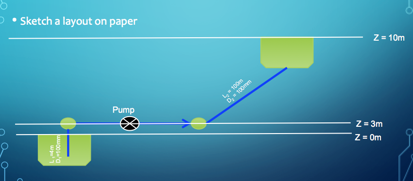
Fig. 28 Schematic of Lift Station
Fig. 28 is a schematic of a pump lifting water through a 100 mm diameter, 100 meter long, ductile iron pipe from a lower to an upper reservoir. The suction side of the pump is a 100 mm diameter, 4-meter long ductile iron pipe. The difference in reservoir free-surface elevations is 10 meters. The pump performance curve is given as
\(h_p = 15 − 0.1Q^2 \)
where the added head is in meters and the flow rate is in liters per second (Lps). The analysis goal is to estimate the flow rate in the system.
To model this situation, the engineer follows the modeling protocol already outlined, only adding the special link.
Convert the image into a bitmap, place the bitmap into a directory where the model input file will be stored.
Start EPA-NET
Set defaults (hydraulics = D-W, units = LPS)
Import the background.
Select the reservoir tool. Put two reservoirs on the map.
Select the node tool, put 2 nodes on the map, these represent the suction and discharge side of the pump.
Select the link (pipe) tool, connect the reservoirs to their nearest nodes.
Select the pump tool.
Connect the nodes to each other using the pump link.
Set the total head each reservoir.
Set the pipe length, roughness height, and diameter in each pipe.
On the Data menu, select Curves. Here is where we create the pump curve. This problem gives the curve as an equation, we will need three points to define the curve. Shutoff (Q = 0), and simple to compute points make the most sense. Fig. 29 illustrates the process for this example.
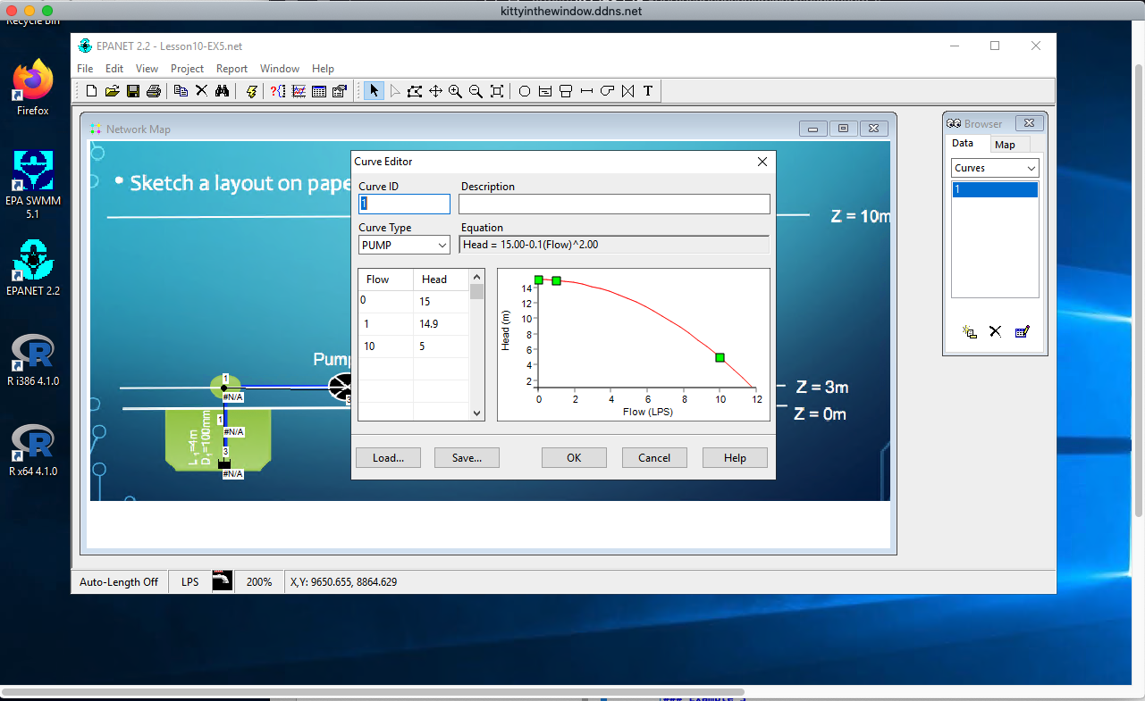
Fig. 29 Pump curve entry dialog box. Three points are entered and the curve equation is created by the program.
Set the pump curve (in the pump dialog). Fig. 30 shows the assignment of pump curve (curve 1) to the pump - failure to assign a curve to a pump (or other curve controlled hydraulic element) is a common mistake leading to error messages in the summary report.
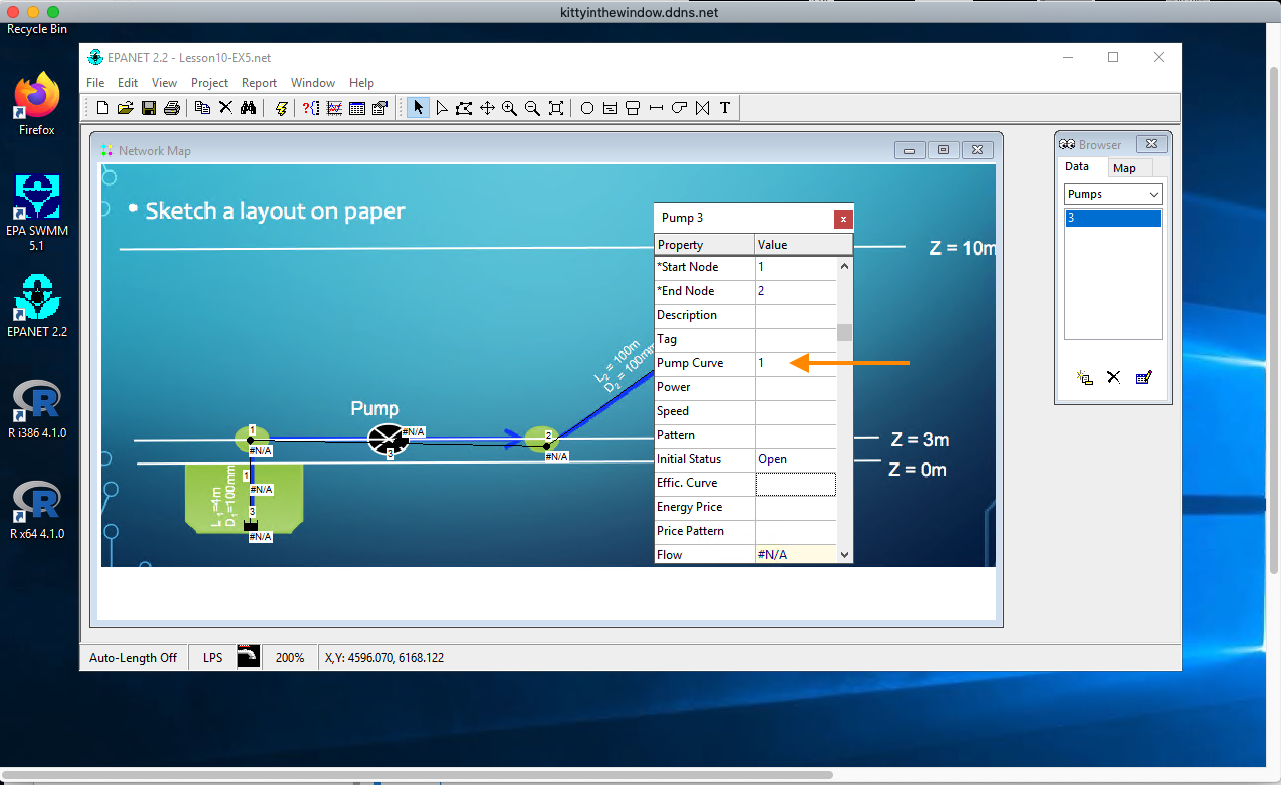
Fig. 30 Pump curve selection.
Save the input file.
Run the program and interpret results as depicted inf Fig. 31.
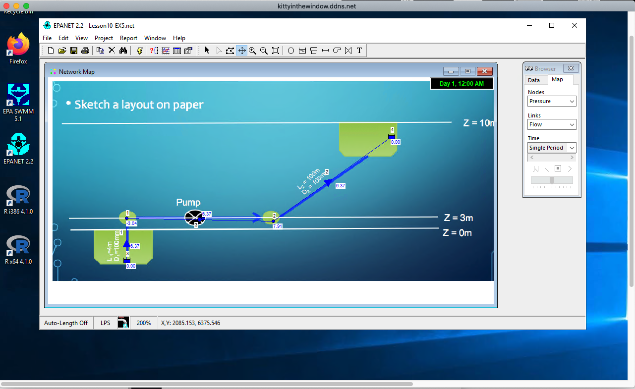
Fig. 31 Example 5 Results
Note
This example was saved as Lesson10-EX5.net on the AWS shared desktop if you wish to run it there. It can also be downloaded from http://54.243.252.9/ce-3372-webroot/EPANET-Files/EX5/EX5.net. The background map is available as http://54.243.252.9/ce-3372-webroot/EPANET-Files/EX5/EX5.bmp as demonstrated in the lecture.
Example 6
Fig. 32 is a water distribution system (skeleton network). The water surface elevation in the storage tank is 315.0 ft.
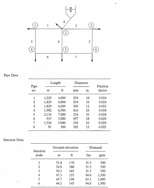
Fig. 32 Exam
Use EPANET and the Darcy-Weisbach head loss model to compute the discharge in each pipe and the pressure at each junction node for the 8-pipe system. Adjust the roughness coefficient (in the program) until the computed friction factors closely agree with the friction factors (exact agreement is not possible) in the table in Fig. 32.
From your model:
Make a screen capture of the EPANET program showing your network map, with the Node ID and Node Pressures displayed on the map, and with the Pipe ID and Pipe Flow Rates on the map.
Make a table that lists each node name, node elevation, and the resultant pressure in U.S. Customary units.
Make a table that lists each pipe name, length, diameter, roughness coefficient, computed friction factor, and the resultant flow rate in U.S. Customary units.
Identify the node with the lowest pressure in your solution.
Note
This example was saved as Lesson10-EX9.net on the AWS shared desktop if you wish to run it there. It can also be downloaded from http://54.243.252.9/ce-3372-webroot/EPANET-Files/EX9/EX9.net. The background map is available as http://54.243.252.9/ce-3372-webroot/EPANET-Files/EX9/EX9.bmp as demonstrated in the lecture.
Example 7
The pipe network in Fig. 32 (shaded part of the diagram in Fig. 33) is expanded to a 14-pipe system and includes a ground-level reservoir near junction node 4 as depicted in Fig. 33.
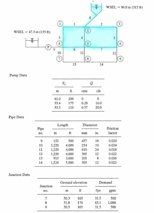
Fig. 33 Exam
The demands at each node in the original system are unchanged.
A pump is installed in the 18-inch diameter pipe extending 500 feet from the ground-level reservoir (WSE = 155 ft.) to junction node 4. The booster pump pushes water into the network; three points on the pump curve are listed on the figure.
Use EPANET and the Darcy-Weisbach head loss model to compute the discharge in each pipe and the pressure at each junction node for the 14-pipe system shown in Fig. 33. Adjust the roughness coefficient (in the program) until the computed friction factors closely agree with the friction factors in the table in Figures 1 and 2, do not expect to obtain an exact match, within 20 percent is sufficient.
Make an table that shows the conversion of the pump curve flow units from cubic-feet-per-second into gallons-per minute.
Make a screen capture of the pump curve input dialog in EPANET and include it (the screen capture) in the technical memorandum below.
Make a screen capture of the EPANET program showing your network map, with the Node ID and Node Pressures displayed on the map, and with the Pipe ID and Pipe Flow Rates on the map. Also set the map features to indicate flow directions on the pipe elements.
Make a table that lists each node name, node elevation, and the resultant pressure in U.S. Customary units.
Make a table that lists each pipe name, length, diameter, computed friction factor, and the resultant flow rate in U.S. Customary units.
Identify the node with the lowest pressure in your solution.
Note
This example was saved as Lesson10-EX8.net on the AWS shared desktop if you wish to run it there. It can also be downloaded from http://54.243.252.9/ce-3372-webroot/EPANET-Files/EX8/EX8.net. The background map is available as http://54.243.252.9/ce-3372-webroot/EPANET-Files/EX8/EX8.bmp as demonstrated in the lecture.
