EPANET Introduction
Course Website
Readings
Cleveland, T.G. (2023). Hydraulic Network Simulation with EPANET and Python. Notes to accompany Metropolia ICT Summer School 2023 Course TX00FJ07 http://freeswmm.ddns.net/ects-epanet/ects-epanet-notes/_build/html/intro.html.
Theodore G. Cleveland, Cristal C. Tay, and Caroline Neale, (2015) EPANET by Example – A How-to-Manual for Network Modeling http://54.243.252.9/ce-3372-webroot/3-Readings/EPANETbyExample/EPANETbyExampleV1.pdf
Cleveland, T. G. (2015) Water Systems Design Notes to Accompany CE 3372 at TTU, Department of Civil, Environmental, and Construction Engineering, Whitacre College of Engineering. http://54.243.252.9/ce-3372-webroot/1-Lessons/Lesson10/PowerPointInLecture/Lecture10.pdf
Hydraulics of Pipelines and Pipe Networks Wurbs, R.A., and James, W. P. (2002) Water Resources Engineering, Prentice Hall; pp.130-156; and 156-198. http://54.243.252.9/ce-3372-webroot/3-Readings/Wurbs130-198/
Pipe Networks Chin, D. (2006). pp. 27-48 in “Water Resources Engineering, 2 ed.” Prentice Hall, Inc. http://54.243.252.9/ce-3372-webroot/3-Readings/Chin_27-48/
Water Distribution Systems “Water Distribution Systems” in Land Development Handbook, Ed. S.O. Dewberry, Dewberry Inc., McGraw-Hill http://54.243.252.9/ce-3372-webroot/3-Readings/WaterDistributionSystems/
Lesson Outline
About EPANET
Installation/FreeSWMM
Example(s)
Flow in a pipe
Flow between two reservoirs
Three-reservoirs to a common junction
Loop network
This lesson is a brief overview of the EPANET software available from the mighty internet, either by download or use the shared version at http://freeswmm.ddns.net.
About EPANET
EPANET is a computer program that performs hydraulics computations in pressure-pipe systems. Most of the problems in the preceding chapters can be solved or well approximated using EPA-NET. The remainder of this lesson shows how to use EPA-NET by a series of representative examples. These examples are at best a subset of the capabilities of the program, but should be enough to get one started. The program requires some hydraulic insight to interpret the results as well as detect data entry or conceptualization errors.
EPANET models are comprised of nodes, links,and reservoirs. Pumps are treated as special links (that add head). Valves are also treated as special links depending on the valve types. All working models must have a reservoir (or storage tank)!
The program has certain defaults that should be set at the beginning of a simulation. The main defaults of importance are the head loss equations (Darcy-Weisbach, Hazen-Williams, or Chezy-Manning) and the flow units (CFS, LPS, etc.)
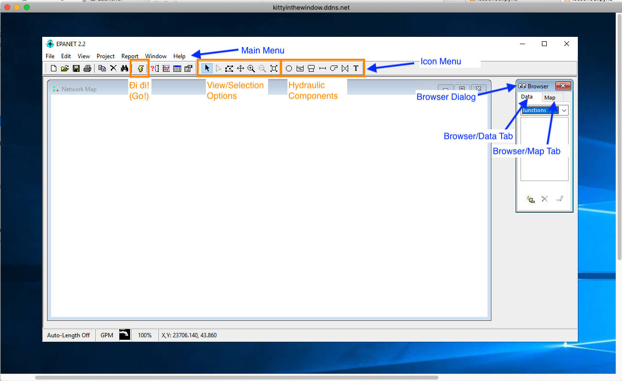
Fig. 15 Annotated GUI Interface
Fig. 15 is an image of the EPANET interface (as supplied by EPA). The annotations are:
Main Menu
Icon Menu
Browser Dialog
Model Drawing Canvass (the big empty area in the figure)
The defaults are set from the main menu in /Project/Defaults then using the tabs in the dialog.
Nodes, reservoirs, tanks, pipes, pumps, and valves are selected from the hydraulic components in the icon menu.
Examples from EPANET by Example
Example 1: Flow in a Single Pipe
The simplest model to consider is from an earlier exercise in the course.
A 5-foot diameter, enamel coated, steel pipe carries \(60^o\)F water at a discharge of 295 cubic-feet per second (cfs).
Using the Moody chart, estimate the head loss in a 10,000 foot length of this pipe.
In EPANET we will start the program, build a tank-pipe system and find the head loss in a 10,000 foot length of the pipe. The program will compute the friction factor for us (and we can check on the Moody chart if we wish).
The main trick in EPA-NET is going to be the friction coefficient, in the EPA-NET manual on page 30 and 31, the author indicates that the program expects a roughness coefficient based on the head loss equation.
The units of the roughness coefficient for a steel pipe are 0.15 × 10⁻³ feet. These can be found from various sources such as Roughness Height On page 71 of the user manual the author states that roughness coefficients are in millifeet (millimeters) when the Darcy-Weisbach head loss model is used. So keeping that in mind we proceed with the example.
The program starts as a blank slate and we will select a reservoir and a node from the tool bar at the top and place these onto the design canvas.
Fig. 16 is a screen capture of the EPA-NET program after setting defaults for the simulation.
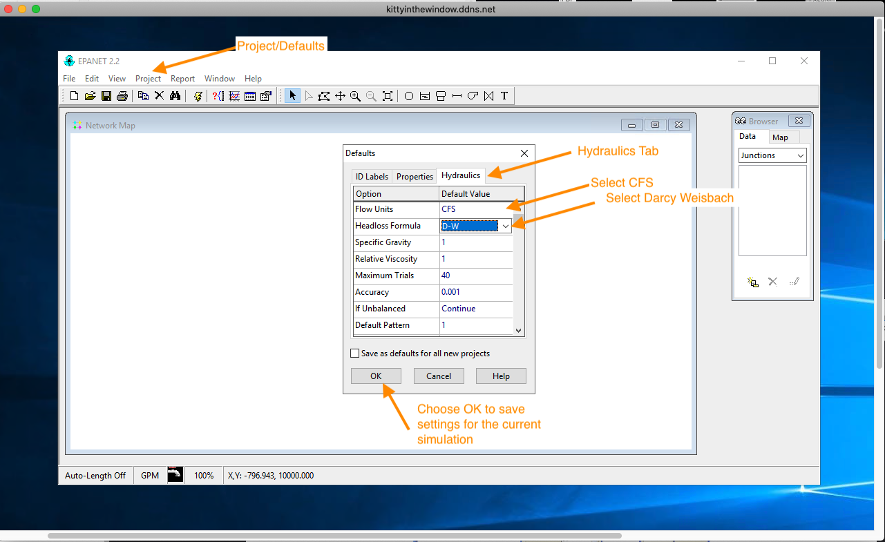
Fig. 16 Set program defaults. In this case units are cubic-feet-per-second and loss model is Darcy-Weisbach.
Failure to set correct units for your problem are sometimes hard to detect (if the model runs), so best to make it a habit to set defaults for all new projects. Next we add the reservoir and nodes as in Fig. 17
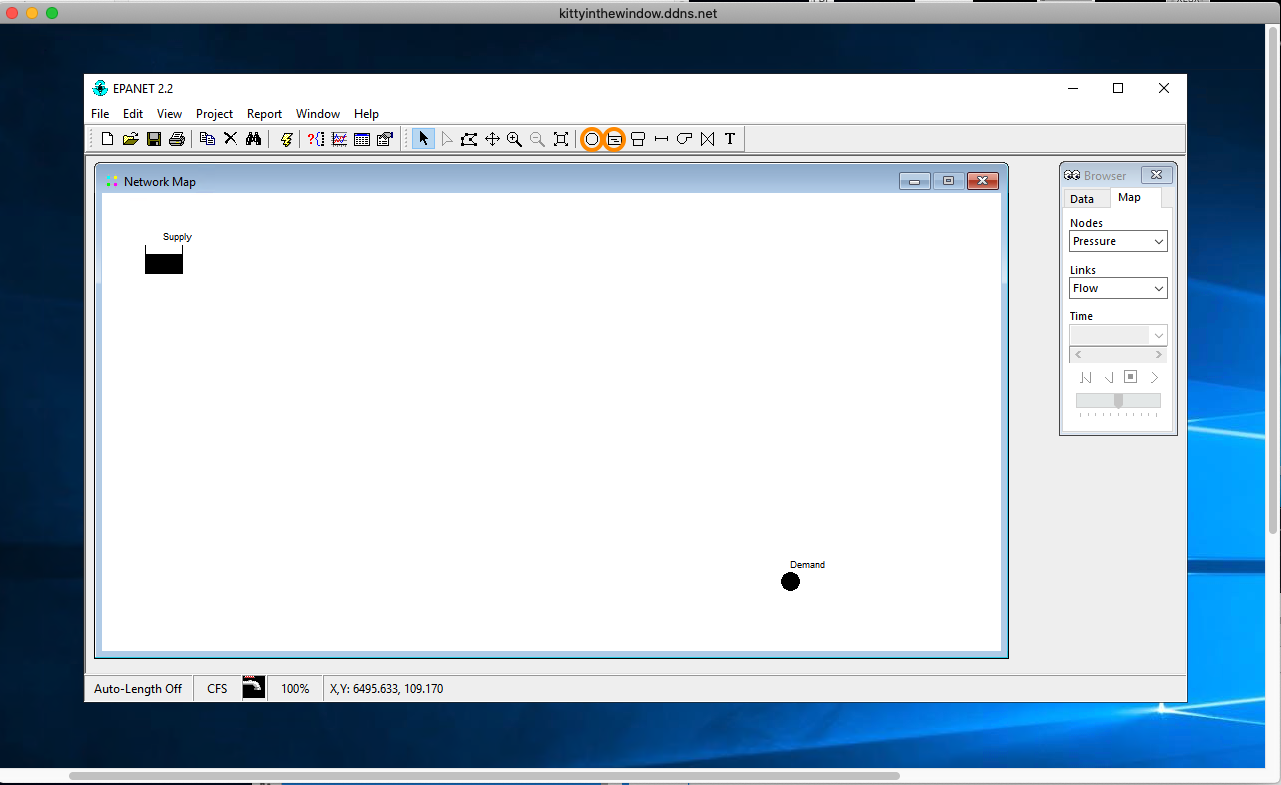
Fig. 17 Place the reservoir and the demand node.
Next we specify a total head at the reservoir (value is unimportant as long as it is big enough to overcome the head loss and not result in a negative pressure at the node) as depicted in Fig. 18
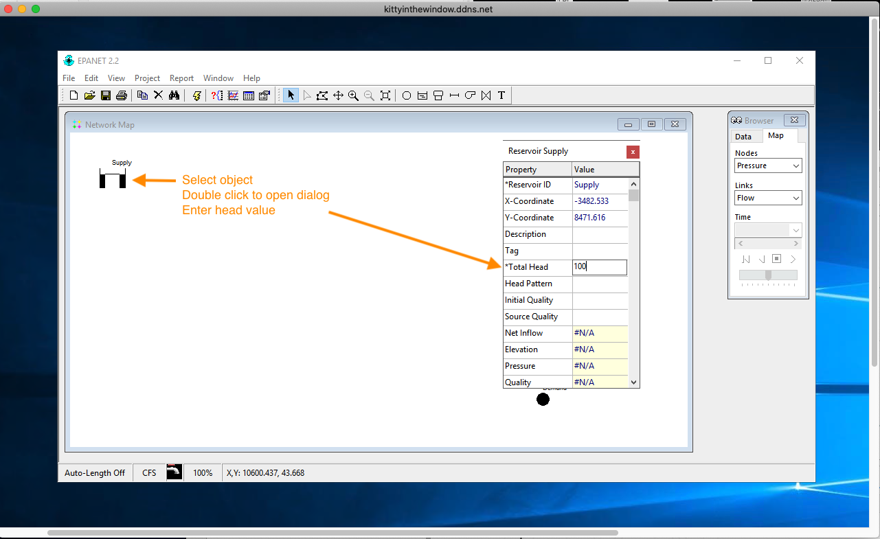
Fig. 18 Set the reservoir total head, 100 feet should be enough in this example.
We will specify the demand at the Demand node equal to the desired flow in the pipe as depicted in Fig. 19.
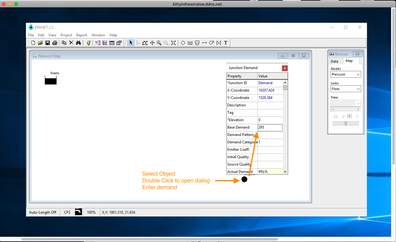
Fig. 19 Set the node elevation and demand. In this case the elevation is set to zero (the datum) and the demand is set to 295 cfs as per the problem statement.
Next we will add the pipe and specify the pipeline properties as in Fig. 20.

Fig. 20 Draw the pipe; set the pipe length, diameter, and roughness height.
The program is now ready to run, next step would be to save the input file (File/Save/Name), then run the program.
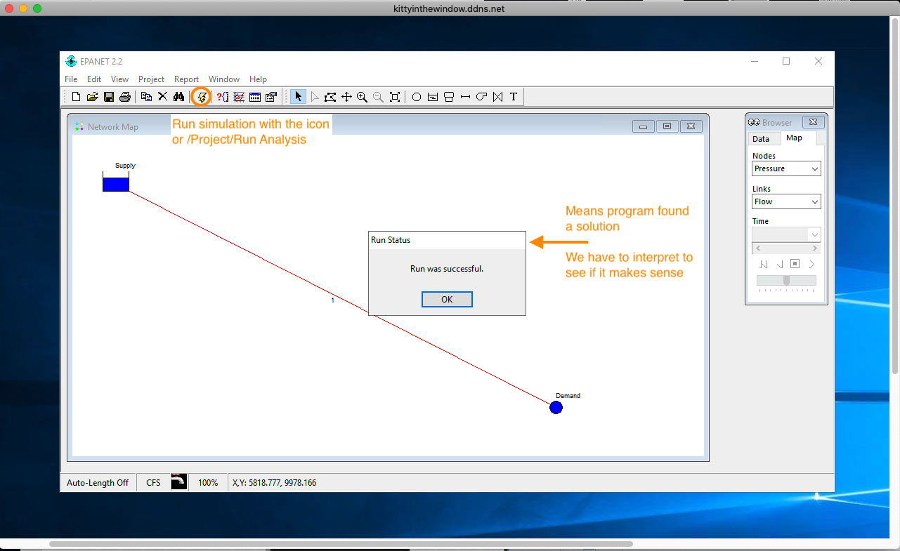
Fig. 21 Running the program
Run the program by selecting the lighting bolt looking thing (kind of channeling Zeus here) and the program will start. If the nodal connectivity is OK and there are no computed negative pressures the program will run. Fig. 21 is the appearance of the program after the run is complete. A successful run means the program found an answer to the problem you provided – whether it is the correct answer to your problem requires the engineer to interpret results and decide if they make sense.
The more common conceptualization errors are incorrect units and head loss equation for the supplied roughness values, missed connections, and forgetting demand somewhere. With practice these kind of errors are straightforward to detect. In the present example we select the pipe and the solution values are reported at the bottom of a dialog box.
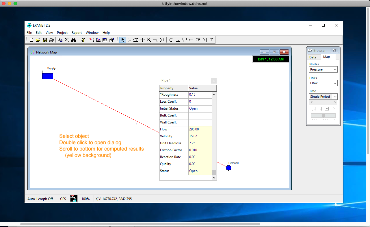
Fig. 22 Solution dialog box for the pipe.
Fig. 22 is the result showing the dialog box for the pipe; the dialog reports about 7.2 feet of head loss per 1000 feet of pipe for a total of 72 feet of head loss in the system. The total head at the demand node is about 28 feet, so the head loss plus remaining head at the node is equal to the 100 feet of head at the reservoir, the anticipated result. The computed friction factor is 0.010, which we could check against the Moody chart if we wished to adjust the model to agree with some other known friction factor.
This “minimal” model has several items common to all EPANET models:
A fixed grade node (reservoir or a tank)
A demand node (all models need at least one to be useful)
A link (in this case a pipe)
Without these three items most models will not run (they are not completely specified models as far as the hydraulic model is concerned).
Note
This example is saved as Lesson9-example1.net on the AWS shared desktop if you wish to run it. It can also be downloaded from URL
Example 2: Flow Between Two Reservoirs
This example represents the situation where the total head is known at two points on a pipeline, and one wishes to determine the flow rate (or specify a flow rate and solve for a pipe diameter). Like the prior example it is contrived, but follows the same general modeling process. As in the prior example, we will use EPA-NET to solve a problem we have already solved by hand.
Using the Moody chart, and the energy equation, estimate the diameter of a cast- iron pipe needed to carry \(60^o\)F water at a discharge of 10 cubic-feet per second (cfs) between two reservoirs 2 miles apart. The elevation difference between the water surfaces in the two reservoirs is 20 feet.
As in the prior example, we will need to specify the pipe roughness terms, then solve by trial- and-error for the diameter required to carry the water at the desired flowrate. Page 31 of the EPA-NET manual suggests that the roughness height for cast iron is 0.85 millifeet, or we could consult Roughness Height
As before the steps to model the situation are:
Start EPA-NET
Set defaults
Select the reservoir tool. Put two reservoirs on the map.
Select the node tool, put a node on the map. EPA NET needs one node!
Select the link (pipe) tool, connect the two reservoirs to the node. One link is the 2 mile pipe, the other is a short large diameter pipe (negligible head loss).
Set the total head each reservoir.
Set the pipe length and roughness height in the 2 mile pipe.
Set the diameter.
Save the input file.
Run the program.
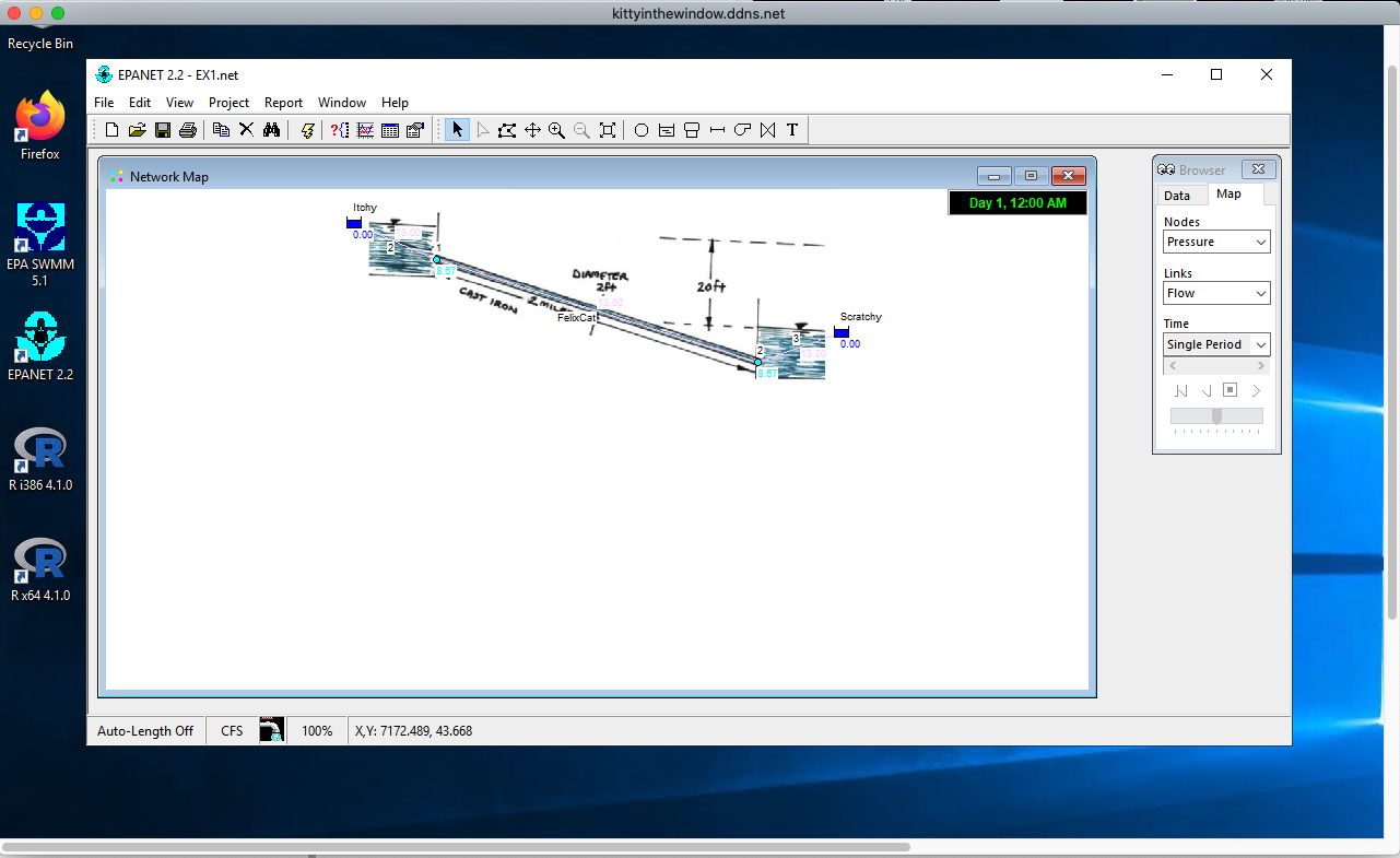
Fig. 23 EPANET screen capture Example 2.
Fig. 23 is a screen capture after the model is built and some trial-and-error diameter selection. Of importance is the node and the “short pipe” that connects the second reservoir.
Note
This example was saved as Lesson8-Example.net on the AWS shared desktop from the “live” demonstration if you wish to run it. It can also be downloaded from http://54.243.252.9/ce-3372-webroot/EPANET-Files/EX1/EX1.net. The background map is available as http://54.243.252.9/ce-3372-webroot/EPANET-Files/EX1/EX1.bmp as demonstrated in the lecture.
Example 3: Three-Reservoirs Connected to a Common Junction
This example repeats another prior problem, but introduces the concept of a basemap (im- age) to help draw the network. First the problem statement
Reservoirs A, B, and C are connected as shown3 in Fig. 24. The water elevations in reservoirs A, B, and C are 100 m, 80 m, and 60 m. The three pipes connecting the reservoirs meet at junction J, with pipe AJ being 900 m long, BJ being 800 m long, and CJ being 700 m long. The diameters of all the pipes are 850 mm. If all the pipes are ductile iron, and the water temperature is 293oK, find the direction and magnitude of flow in each pipe.
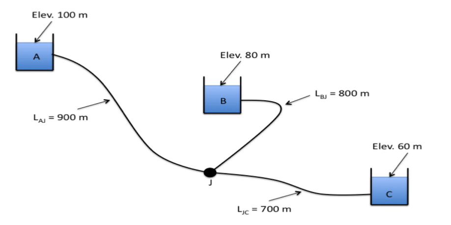
Fig. 24 Basemap for Example 3
Here we will first convert the image into a bitmap (.bmp) file so EPANET can import the background image and we can use it to help draw the network. The remainder of the problem is reasonably simple and is an extension of the previous problem.
The steps to model the situation are:
Convert the image into a bitmap, place the bitmap into a directory where the model input file will be stored.
Start EPA-NET
Set defaults
Import the background.
Select the reservoir tool. Put three reservoirs on the map.
Select the node tool, put the node on the map.
Select the link (pipe) tool, connect the three reservoirs to the node.
Set the total head each reservoir.
Set the pipe length, roughness height, and diameter in each pipe.
Save the input file.
Run the program.
Fig. 25 is the result of the above steps. In this case the default units were changed to LPS (liters per second). The roughness height is about 0.26 millimeters (if converted from the 0.85 millifeet unit).
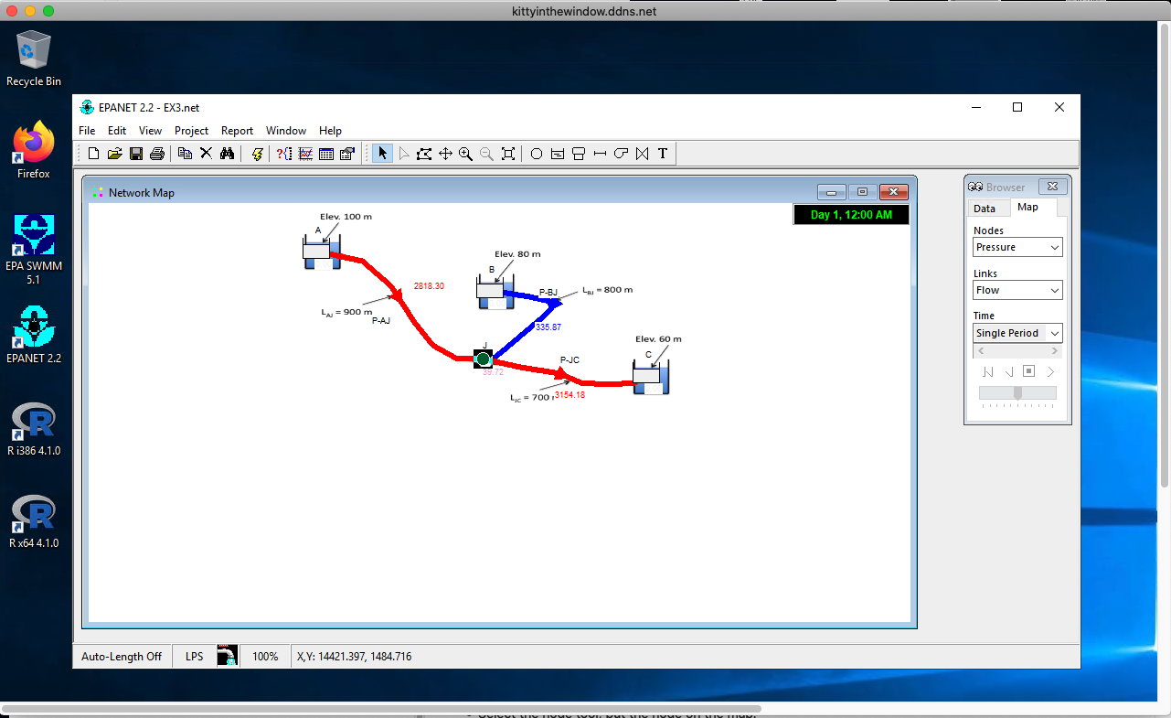
Fig. 25 Results for Example 3
Note
This example was saved as Lesson9-EX3.net on the AWS shared desktop if you wish to run it there. It can also be downloaded from http://54.243.252.9/ce-3372-webroot/EPANET-Files/EX3/EX3.net. The background map is available as http://54.243.252.9/ce-3372-webroot/EPANET-Files/EX3/EX3.bmp as demonstrated in the lecture.
Example 4: A Simple Network
Expanding the examples, we will next consider a looped network. As before we will use a prior exercise as the motivating example.
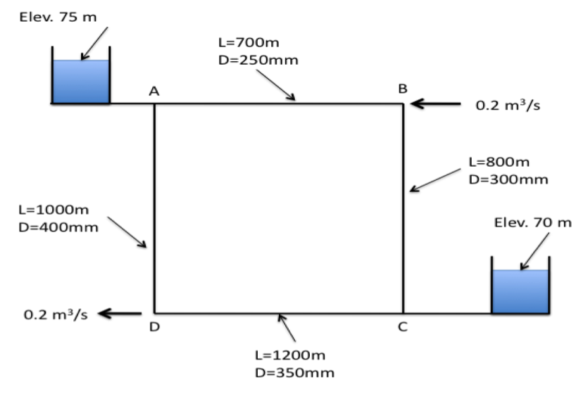
Fig. 26 Basemap for Example 4
The water-supply network shown in Fig. 26 has constant-head elevated storage tanks at A and C, with inflow and outflow at B and D. The network is on flat terrain with node elevations all equal to 50 meters If all pipes are ductile iron, compute the inflows/outflows to the storage tanks. Assume that flow in all pipes are fully turbulent.
As before we will follow the modeling protocol but add demand at the nodes. The steps to model the situation are:
Convert the image into a bitmap, place the bitmap into a directory where the model input file will be stored.
Start EPA-NET
Set defaults
Import the background.
Select the reservoir tool. Put two reservoirs on the map.
Select the node tool, put 4 nodes on the map.
Select the link (pipe) tool, connect the reservoirs to their nearest nodes. Connect the nodes to each other.
Set the total head each reservoir.
Set the pipe length, roughness height, and diameter in each pipe. The pipes that connect to the reservoirs should be set as short and large diameter, we want negligible head loss in these pipes so that the reservoir head represents the node heads at these locations.
Save the input file.
Run the program.
In this case the key issues are the units (liters per second) and roughness height (0.26 millimeters).
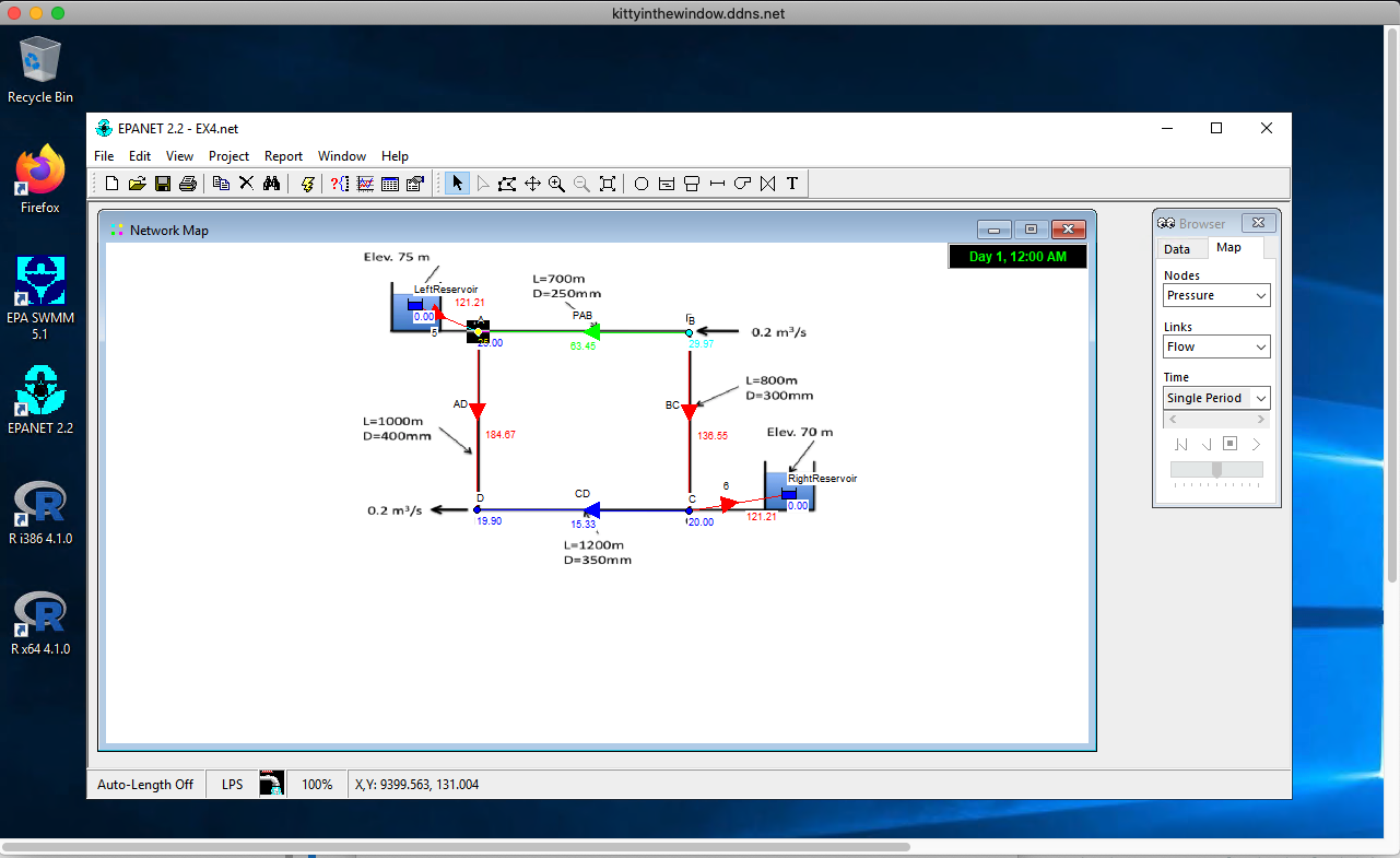
Fig. 27 Results for Example 4
Fig. 27 is a screen capture of a completed model.
Note
This example was saved as Lesson9-EX3.net on the AWS shared desktop if you wish to run it there. It can also be downloaded from http://54.243.252.9/ce-3372-webroot/EPANET-Files/EX4/EX4.net. The background map is available as http://54.243.252.9/ce-3372-webroot/EPANET-Files/EX4/EX4.bmp as demonstrated in the lecture.
