Analytical Models with Decay and Adsorbtion
This section is incomplete - saved for future semester
import math
from scipy.special import erf, erfc

def c2adrl(conc0, distx, disty, dispx, dispy, velocity, time, lenY, retardation, _lambda):
    vadj = velocity / retardation
    dispXadj = dispx / retardation
    dispYadj = dispy / retardation
    lambadj = _lambda / retardation

    uuu = math.sqrt(1.0 + 4.0*lambadj*dispXadj/vadj)
    ypp = (disty + 0.5*lenY) / (2*math.sqrt(dispYadj*distx))
    ymm = (disty - 0.5*lenY) / (2*math.sqrt(dispYadj*distx))

    arg1 = (distx - vadj*time*uuu) / (2*math.sqrt(dispXadj*vadj*time))
    arg2 = (distx / (2*dispXadj)) * (1 - uuu)

    term0 = conc0 / 4
    term1 = math.exp(arg2)
    term2 = erfc(arg1)
    term3 = (erf(ypp) - erf(ymm))

    c2adrl = term0 * term1 * term2 * term3
    return c2adrl
# inputs
c_initial = 100.0
xx = 100
yy = 5
Dx = 1.0
Dy = 0.1
V = 1.0
time = 10.0
Y = 10.0
R = 1.0
LAM = 0.00001
output=c2adrl(c_initial, xx, yy, Dx, Dy, V, time, Y, R, LAM)
print("x= ",round(xx,2)," y= ",round(yy,2)," t= ",round(time,1)," C(x,y,t) = ",round(output,3))
# make a plot
x_max = 400
y_max = 20
# build a grid
nrows = 50
deltax = (x_max)/nrows
x = []
x.append(1)
for i in range(nrows):
if x[i] == 0.0:
x[i] = 0.00001
x.append(x[i]+deltax)
ncols = 50
deltay = (y_max*2)/(ncols-1)
y = []
y.append(-y_max)
for i in range(1,ncols):
if y[i-1] == 0.0:
y[i-1] = 0.00001
y.append(y[i-1]+deltay)
#y
#y = [i*deltay for i in range(how_many_points)] # constructor notation
#y[0]=0.001
ccc = [[0 for i in range(nrows)] for j in range(ncols)]
for jcol in range(ncols):
for irow in range(nrows):
ccc[irow][jcol] = c2adrl(c_initial, x[irow], y[jcol], Dx, Dy, V, time, Y, R, LAM)
#y
my_xyz = [] # empty list
count=0
for irow in range(nrows):
for jcol in range(ncols):
my_xyz.append([ x[irow],y[jcol],ccc[irow][jcol] ])
# print(count)
count=count+1
#print(len(my_xyz))
import pandas
my_xyz = pandas.DataFrame(my_xyz) # convert into a data frame
import numpy
import matplotlib.pyplot
from scipy.interpolate import griddata
# extract lists from the dataframe
coord_x = my_xyz[0].values.tolist() # column 0 of dataframe
coord_y = my_xyz[1].values.tolist() # column 1 of dataframe
coord_z = my_xyz[2].values.tolist() # column 2 of dataframe
#print(min(coord_x), max(coord_x)) # activate to examine the dataframe
#print(min(coord_y), max(coord_y))
coord_xy = numpy.column_stack((coord_x, coord_y))
# Set plotting range in original data units
lon = numpy.linspace(min(coord_x), max(coord_x), 64)
lat = numpy.linspace(min(coord_y), max(coord_y), 64)
X, Y = numpy.meshgrid(lon, lat)
# Grid the data; use linear interpolation (choices are nearest, linear, cubic)
Z = griddata(numpy.array(coord_xy), numpy.array(coord_z), (X, Y), method='cubic')
# Build the map
fig, ax = matplotlib.pyplot.subplots()
fig.set_size_inches(14, 7)
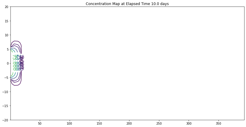
CS = ax.contour(X, Y, Z, levels = [1,5,10,25,50,75,100])
ax.clabel(CS, inline=2, fontsize=16)
ax.set_title('Concentration Map at Elapsed Time '+ str(round(time,1))+' days');
x= 100 y= 5 t= 10.0 C(x,y,t) = 0.0