
22. Stormwater Conduit Sizing#
Course Website
Readings#
Videos#
Scripts/Spreadsheets#
Storm Sewers#
Storm sewers are an essential component of urban drainage systems, designed to manage the runoff generated by rainfall events. Unlike sanitary sewers, which carry wastewater, storm sewers convey rainwater and surface runoff away from streets, parking lots, and other impervious surfaces to prevent flooding and waterlogging in urban areas. These systems typically consist of a network of inlets, underground pipes, manholes, and outfalls that discharge water into nearby water bodies such as rivers, lakes, or retention basins. Properly designed storm sewer systems help reduce flood risks, protect infrastructure, and improve safety by minimizing surface water accumulation during storms.
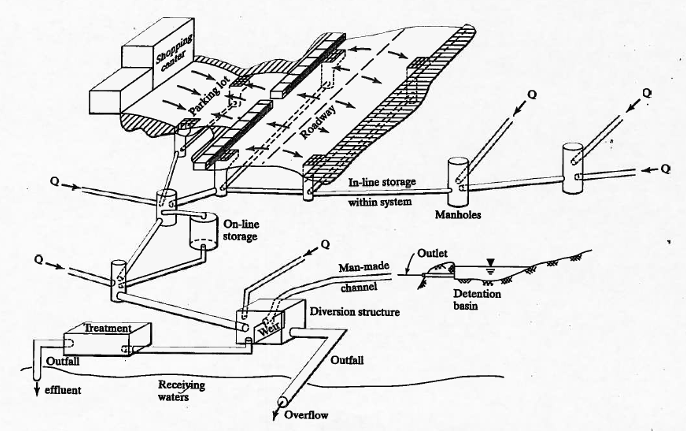
Storm Sewer Components
Inlets to capture runoff
Conduits to convey to outfall
Lift Stations if cannot gravity flow to outfall
Detention and diversions
Outfalls release water back into environment
Hydrological Considerations in Storm Sewer Design#
Storm sewer design requires careful consideration of various hydrological factors to ensure the system can handle anticipated runoff volumes and flow rates. Some of the key hydrological aspects include:
Rainfall Intensity and Duration: The design process begins with an analysis of rainfall data, often based on intensity-duration-frequency (IDF) curves. These curves help determine the intensity and duration of rainfall events that the storm sewer system should be able to manage. Engineers typically design for specific return periods, such as a 10-year or 100-year storm event, depending on local regulations and the level of protection required. (We have already examined these topics!)
Runoff Coefficients: Runoff coefficients represent the fraction of rainfall that becomes surface runoff. These coefficients vary based on the type of land cover (e.g., impervious surfaces like roads and rooftops, or pervious areas like parks and gardens). The more impervious the area, the higher the runoff coefficient, which results in greater volumes of stormwater entering the system. (We have examined runoff generation via Unit Hydrographs as well as rational method)
Watershed Characteristics: The size, slope, and shape of the drainage area (watershed) contribute to how quickly and how much water will enter the storm sewer system. Steeper slopes typically lead to faster runoff, while larger watersheds generate greater volumes of water. These characteristics influence the required capacity of storm sewers. (The whole point of delineation, and path identification)
Time of Concentration: This is the time it takes for runoff to travel from the furthest point in the watershed to the storm sewer inlet. The time of concentration affects the peak flow rate that the system must handle. Shorter times of concentration generally lead to higher peak flows. (Synthetic unit hydrographs)
Peak Flow Estimation: Hydrologists use methods such as the Rational Method or more complex hydrological models to estimate the peak flow rate that storm sewers will need to convey. Peak flow is critical in determining the diameter of pipes and the placement of inlets to avoid overloading the system.
Infiltration and Storage: In some cases, designers incorporate infiltration or storage solutions (such as detention basins or permeable pavements) to reduce the volume and speed of water entering the storm sewer. This mitigates the risk of overwhelming the system during heavy rainfall events. (Why we model things!)
Note
There is a whole set of hydraulic concerns, these are generally handled contemporanously (at the same time) in design and analysis.
A Rational Method for Storm Sewer Conduit Sizing#
The Rational Method is a widely used, straightforward approach for sizing storm sewer conduits and estimating stormwater runoff, particularly in urban drainage design. It is used to obtain initial estimates of conduit diameters, flowlines, and hydraulic grade lines for storm sewer systems. Although more advanced hydrologic models are available, the Rational Method remains popular for preliminary design due to its simplicity and ease of application, especially when dealing with small catchments. Overview of the Rational Method
The Rational Method estimates peak runoff from a given watershed using the formula:
\(Q=CIA\)
Where:
\(Q\) = Peak runoff rate (cubic feet per second or cfs), \(C\) = Runoff coefficient (dimensionless), representing the portion of rainfall that becomes surface runoff, \(I\) = Rainfall intensity (inches per hour), determined based on the design storm and time of concentration for the watershed, \(A\) = Drainage area (acres).
Steps for Storm Sewer Conduit Sizing Using the Rational Method#
Determine the Design Storm Event: Identify the design storm return period (e.g., 5-year, 10-year, or 100-year storm) based on local regulations or standards. This helps establish the rainfall intensity (II) for the design.
Estimate the Time of Concentration: The time of concentration (\(T_C\)) is the time it takes for runoff to travel from the most distant point of the catchment to the outlet or point of interest. Several empirical methods (e.g., Kirpich’s equation) can be used to calculate this value.
Select the Runoff Coefficient (C): The runoff coefficient is chosen based on the land cover within the drainage area. For example, impervious surfaces (like pavement) will have a higher C value (around 0.9), while pervious surfaces (like grassland) will have a lower value (around 0.2). Mixed land uses are weighted to determine an appropriate CC value for the entire catchment.
Calculate Peak Runoff (\(Q_P\)): Using the Rational Method equation, the peak runoff \(Q_P\) is calculated by multiplying the runoff coefficient CC, the rainfall intensity \(I\), and the drainage area AA.
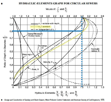
Conduit Sizing: Once the peak runoff \(Q_P\) is determined, the required diameter of the storm sewer conduit can be estimated using Manning’s equation for open channel flow, assuming the conduit is flowing full or partially full. Manning’s equation is:
\(Q=\frac{1.49}{n}AR^{2/3}S_0^{1/2}\)
Where:
\(Q\) = Discharge (cfs),
\(n\) = Manning’s roughness coefficient (dimensionless),
\(A\) = Cross-sectional area of flow (square feet),
\(R\) = Hydraulic radius (feet),
\(S_0\) = Slope of the conduit (ft/ft).
The required pipe diameter can be determined iteratively by solving Manning’s equation for AA and matching it with the calculated peak runoff \(Q\).
Hydraulic Grade Line (HGL) and Flowline: The Hydraulic Grade Line (HGL) represents the level to which water would rise in open vertical tubes attached to the conduit. It is used to assess the system’s capacity to convey flow without excessive pressure buildup. The flowline refers to the bottom elevation of the pipe at various points along the system. These elevations are crucial for ensuring gravity flow and preventing backflow within the system.
To approximate the HGL by hand, designers often check that the conduit slope and size provide sufficient capacity by comparing the HGL with the energy grade line (EGL), which accounts for both the potential and kinetic energy within the system. By adjusting the pipe size or slope, the designer ensures the HGL stays within acceptable bounds.
Advantages of the Rational Method#
Simplicity: The Rational Method is straightforward and can be applied manually without requiring complex computer simulations, making it useful for small drainage areas.
Preliminary Design: It provides a good starting point for conduit sizing, helping designers quickly estimate pipe diameters, slopes, and flowlines before conducting more detailed hydraulic analyses.
Applicability for Urban Settings: The method is particularly suited for urban environments with impervious surfaces, where runoff behavior is more predictable.
Limitations of the Rational Method#
Small Catchment Limitation: The Rational Method is typically recommended for small watersheds (less than 200 acres) because it assumes uniform rainfall distribution and runoff response, which may not hold in larger or more complex watersheds.
Peak Flow Only: It estimates only the peak runoff rate and does not provide information about the full runoff hydrograph (i.e., the variation of flow over time).
Constant Runoff Coefficient: The method assumes a constant runoff coefficient \(C\), which may vary during a storm event due to factors like soil saturation or changing land cover conditions.
Summary#
The Rational Method provides a practical, by-hand approach for obtaining initial estimates of conduit diameters, flowlines, and hydraulic grade lines for storm sewer systems. It serves as a preliminary design tool, ensuring that designers can evaluate the capacity and size of storm sewer conduits before engaging in more sophisticated analyses, making it an essential tool in urban stormwater management.
Design Example#
Conduits convey Flow from one location to another
Pipes
Culverts
Open channels
Design objectives are to select:
Size
Material, and
Slope (velocity control)
Conduit size (diameter) is dictated by
Flow required
Burial depth relative to drop available
A good preliminary design can be obtained using a combination of the rational equation and manning’s equation
Done without regard to downstream boundary conditions
Needs to be checked using a hydraulic model (like SWMM)
Determine discharge in each pipe using hydrologic estimates (rational method)
Size the conduit using Manning’s equation
Data Required:
Layout of system
Drainage area and Junction/Inlet locations
Pipe alignments
Outfall location
Land surface elevations
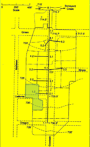
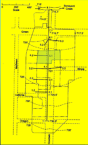
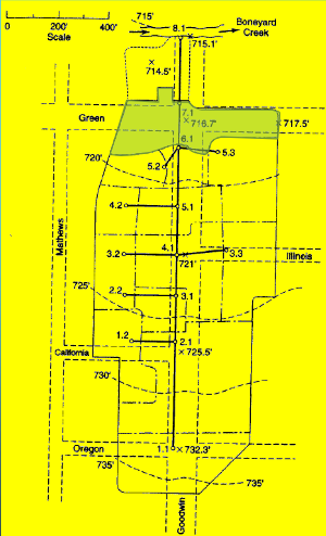
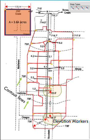
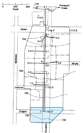
Drainage Area 1.1#
Identify the individual drainage area(s) for analysis
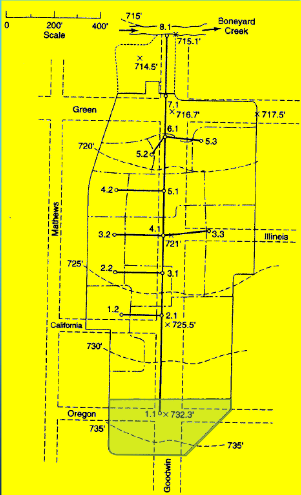
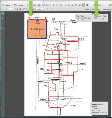
Measure area(s) using appropriate tools; to determine the area of each contributing area, in acres. (G3DATA; PLANIMETER, etc).
Area = 1.50*3.67/2.43 = 2.26 acres (using Acrobat Pro and a conversion ratio 2.43 in^2 => 3.67 acres)
Estimate a runoff coefficient (table look-up)
C = 0.65
Estimate \(T_c\) surface flow to inlet/junction.
Measure actual best-guess flow path(s)
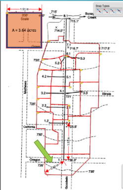
Find Slope (737.5 – 732.3)/(0.92*400/1.51) = 5.2ft/243.7 ft = 0.021 (2.1%) from elevation mapping.
Determine some kind of cover.
Apply NRCS Velocity, NRCS Upland, or Kerby-Kirpich.
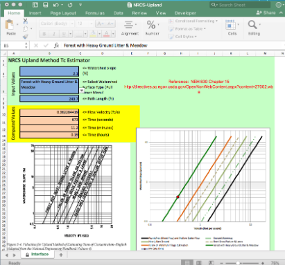
Use method that makes most sense consistent with locale.
Repeat for each area.
Estimate \(T_c\) all connecting routes to junction. (Need to measure pipe lengths before this calculation - shown after all the areas in this document)
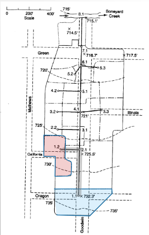
Drainage Area 1.2#
Measure area(s) using appropriate tools; to determine the area of each contributing area, in acres. (G3DATA; PLANIMETER, etc).
Area = 0.84*3.67/2.43 = 1.26 acres (using Acrobat Pro and a conversion ratio 2.43 in^2 => 3.67 acres)
Estimate a runoff coefficient (table look-up)
C = 0.80
Estimate \(T_c\) surface flow to inlet.
Estimate \(T_c\) all connecting routes to junction.
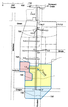
Drainage Area 2.1#
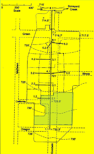
Measure area(s) using appropriate tools; to determine the area of each contributing area, in acres. (G3DATA; PLANIMETER, etc).
Area = 2.58*3.67/2.43 = 3.89 acres (using Acrobat Pro and a conversion ratio 2.43 in^2 => 3.67 acres)
Estimate a runoff coefficient (table look-up)
C = 0.70
Estimate \(T_c\) surface flow to inlet.
Estimate \(T_c\) all connecting routes to junction.
Drainage Area 2.2#
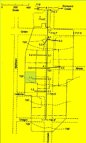
Measure area(s) using appropriate tools; to determine the area of each contributing area, in acres. (G3DATA; PLANIMETER, etc).
Area = 0.35*3.67/2.43 = 0.53 acres (using Acrobat Pro and a conversion ratio 2.43 in^2 => 3.67 acres)
Estimate a runoff coefficient (table look-up)
C = 0.80
Estimate \(T_c\) surface flow to inlet.
Estimate \(T_c\) all connecting routes to junction.
Drainage Area 3.1#
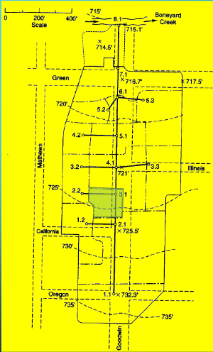
Measure area(s) using appropriate tools; to determine the area of each contributing area, in acres. (G3DATA; PLANIMETER, etc).
Area = 0.45*3.67/2.43 = 0.68 acres (using Acrobat Pro and a conversion ratio 2.43 in^2 => 3.67 acres)
Estimate a runoff coefficient (table look-up)
C = 0.70
Estimate \(T_c\) surface flow to inlet.
Estimate \(T_c\) all connecting routes to junction.
Drainage Area 3.2#
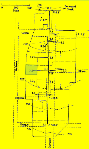
Measure area(s) using appropriate tools; to determine the area of each contributing area, in acres. (G3DATA; PLANIMETER, etc).
Area = 0.30*3.67/2.43 = 0.45 acres (using Acrobat Pro and a conversion ratio 2.43 in^2 => 3.67 acres)
Estimate a runoff coefficient (table look-up)
C = 0.85
Estimate \(T_c\) surface flow to inlet.
Estimate \(T_c\) all connecting routes to junction.
Drainage Area 3.3#
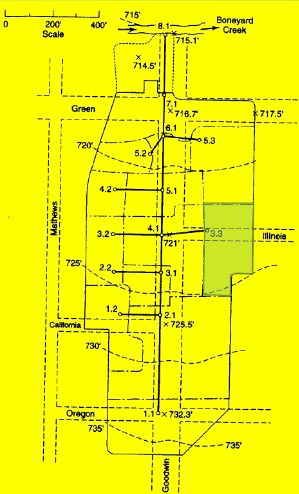
Measure area(s) using appropriate tools; to determine the area of each contributing area, in acres. (G3DATA; PLANIMETER, etc).
Area = 1.05*3.67/2.43 = 1.58 acres (using Acrobat Pro and a conversion ratio 2.43 in^2 => 3.67 acres)
Estimate a runoff coefficient (table look-up)
C = 0.65
Estimate \(T_c\) surface flow to inlet.
Estimate \(T_c\) all connecting routes to junction.
Drainage Area 4.1#
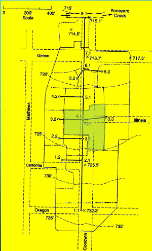
Measure area(s) using appropriate tools; to determine the area of each contributing area, in acres. (G3DATA; PLANIMETER, etc).
Area = 1.33*3.67/2.43 = 2.01 acres (using Acrobat Pro and a conversion ratio 2.43 in^2 => 3.67 acres)
Estimate a runoff coefficient (table look-up)
C = 0.75
Estimate \(T_c\) surface flow to inlet.
Estimate \(T_c\) all connecting routes to junction.
Drainage Area 4.2#
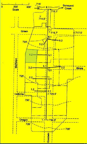
Measure area(s) using appropriate tools; to determine the area of each contributing area, in acres. (G3DATA; PLANIMETER, etc).
Area = 0.44*3.67/2.43 = 0.66 acres (using Acrobat Pro and a conversion ratio 2.43 in^2 => 3.67 acres)
Estimate a runoff coefficient (table look-up)
C = 0.85
Estimate \(T_c\) surface flow to inlet.
Estimate \(T_c\) all connecting routes to junction.
Drainage Area 5.1#
Measure area(s) using appropriate tools; to determine the area of each contributing area, in acres. (G3DATA; PLANIMETER, etc).
Area = 0.78*3.67/2.43 = 1.17 acres (using Acrobat Pro and a conversion ratio 2.43 in^2 => 3.67 acres)
Estimate a runoff coefficient (table look-up)
C = 0.70
Estimate \(T_c\) surface flow to inlet.
Estimate \(T_c\) all connecting routes to junction.
Drainage Area 5.2#
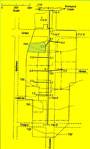
Measure area(s) using appropriate tools; to determine the area of each contributing area, in acres. (G3DATA; PLANIMETER, etc).
Area = 0.44*3.67/2.43 = 0.66 acres (using Acrobat Pro and a conversion ratio 2.43 in^2 => 3.67 acres)
Estimate a runoff coefficient (table look-up)
C = 0.65
Estimate \(T_c\) surface flow to inlet.
Estimate \(T_c\) all connecting routes to junction.
Drainage Area 5.3#
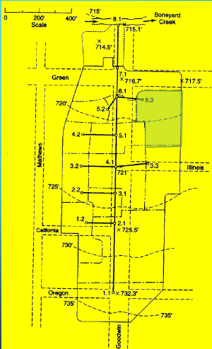
Measure area(s) using appropriate tools; to determine the area of each contributing area, in acres. (G3DATA; PLANIMETER, etc).
Area = 1.16*3.67/2.43 = 1.75 acres (using Acrobat Pro and a conversion ratio 2.43 in^2 => 3.67 acres)
Estimate a runoff coefficient (table look-up)
C = 0.55
Estimate \(T_c\) surface flow to inlet.
Estimate \(T_c\) all connecting routes to junction.
Drainage Area 6.1#
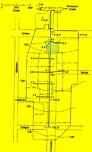
Measure area(s) using appropriate tools; to determine the area of each contributing area, in acres. (G3DATA; PLANIMETER, etc).
Area = 0.36*3.67/2.43 = 0.54 acres (using Acrobat Pro and a conversion ratio 2.43 in^2 => 3.67 acres)
Estimate a runoff coefficient (table look-up)
C = 0.75
Estimate \(T_c\) surface flow to inlet.
Estimate \(T_c\) all connecting routes to junction.
Drainage Area 7.1#
Measure area(s) using appropriate tools; to determine the area of each contributing area, in acres. (G3DATA; PLANIMETER, etc).
Area = 1.44*3.67/2.43 = 2.17 acres (using Acrobat Pro and a conversion ratio 2.43 in^2 => 3.67 acres)
Estimate a runoff coefficient (table look-up)
C = 0.70
Estimate \(T_c\) surface flow to inlet.
Estimate \(T_c\) all connecting routes to junction.
Identify and measure conduit lengths#
Use appropriate tool to measure distances between Node ID (Acrobat Pro in the figure)
Select distance tool
Measure the 400 foot scale
Save scale factor: 1.51 in == 400 feet
Then measure length each pipe, convert to appropriate units.
Pipe P 1.1:
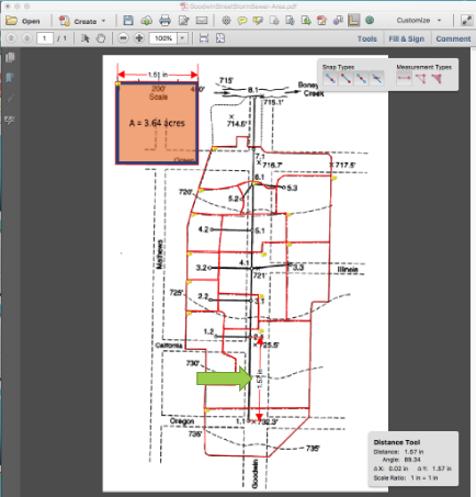
Connects 1.1 to 2.1 (need this linkage later on)
Length = 1.57*400/1.51 = 415 ft
Repeat for all the other pipes, store results somewhere convienient.
Build a spreadsheet with the information
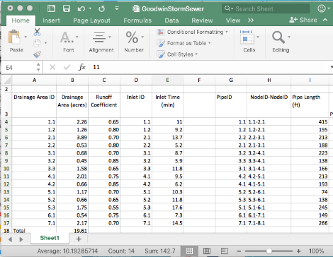
Note the naming convention (a bit awkward above, but faithful to the original example)
Compute Pipe Slopes#
Note
Either during the length measurements or now, record junction elevations, and use these to estimate initial pipe slopes – the pipe slopes and diameters are ultimately the only design controls we can actually engineer – so need a starting point.
Here the 3D nature of the design begins to manifest!
Again employ a suitable tool such as Acrobat Pro, and use the node elevations and topographic map to estimate pipe slopes.
The pipes are usually buried, so we will be able to change slopes somewhat in the plan and profile drawings to maintain suitable hydraulic behavior. Add these slopes to the spreadsheed for each pipe.
Intensity (as an) Equation#
Next we will need to precipitation information for the design.
Easiest for this example is to build an IDF curve for the location.
The basin in the example is in Urbana, Illinois – Use NOAA Atlas 14
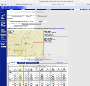
For the example use a 2-yr ARI
Download the table
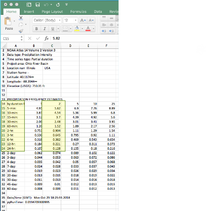
Use the 2-nd column
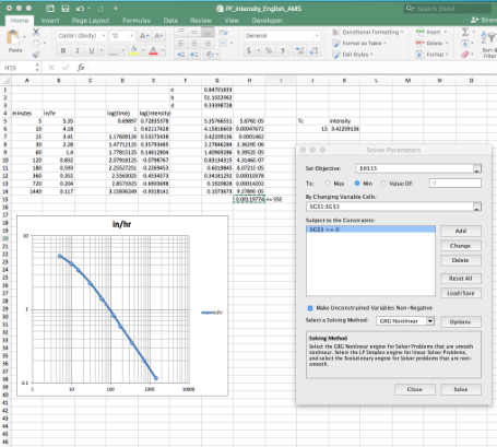
Use solver to fit
\(I = \frac{B}{(T_c + D)^E}\)These E,B,D are unknowns, we are fitting the equation to the NOAA values and \(T_c\) (as a variable) to recover a model (which we call an IDF curve)
Use this equation for estimating intensity and runoff
Intensity function for the example is:
\(I = \frac{54.82}{(T_c + 9.21)^{0.884}}\)
This equation can be coded into an analysis spreadsheet directly, then used to size the pipes.
Estimate Discharge in Each Conduit#
Size using Manning’s Equation rearranged to solve for diameter (US Customary Units)
\(Q=1.333(\frac{Qn}{\sqrt{S}})^{3/8}\)Assumes pipes are full, but they will have a free surface at the design discharge.
Start at most upstream point, apply rational method to the area that drains to the upstream junction/inlet.
This is the discharge in the first pipe. Then
Check velocity criteria.
Determine pipe travel time to next node from discharge.
\(V=\frac{Q}{n}R^{2/3}\sqrt{S}\)Repeat for all the terminal/origin nodes.
At a junction/inlet that collects both from local inlet, and upstream pipe
Choose larger of
local inlet time
upstream inlet time + travel time
Use the selected time to compute intensity all areas to the junction
\(Q_p = CA_{local}+\sum CA_{all upstream}\)
Size pipe leaving the junction by this discharge; move to the next downstream node and repeat.
Continue downstream in same fashion until reach outfall
Accumulate \(CA\) values and \(T_c\) as you move downstream in the design (saves time).
Check that areas all acucmulate correctly
\(T_c\) should be increasing in value as you move downstream
When you reach the outfall you should have:
Pipe sizes
Pipe discharges
Next check the hydraulics
SWMM – Enter \(Q_{inlet}\) directly and check the pipe hydraulics
SWMM – Approximate the rational method in SWMM to check a design hyetograph.
Use SWMM results to adjust the design, and produce a hydraulic grade line drawing (the profile part of plan and profile drawing)
Now use inlet design tools to size the inlets.