
4. Demand Estimation#
Course Website
Demand estimates are required to size water systems to meet some purpose, or establish that the particular system is infeasible.
Warning
This section is incomplete
Readings#
Additional Readings
Gupta, R. S. 2017. Hydrology and Hydraulic Systems. Waveland Press, Inc. pp 1-19
Land Development Handbook 4ed. 2019. The most useful $200 you will spend in Civil Engineering - this is an upgrade to the copy I used for the excerpt above. If you buy one get a physcial book - they don’t break, work anytime the lights are on, and you can use it for squashing bugs.
Frauenthal, J.C. 1980. Introduction to Population Modeling. Birkhäuser, Boston. (Internet Archive has a copy one can borrow, but no free PDFs on the mighty internet)
Steel E. W. and McGhee, TJ (1979), Water Supply and Sewerage, Mcgraw-hill, inc., new york. I think this is a scan of a first edition. Second author has a 6th edition, same title circa 1991.
Videos#
Lesson Outline#
topic1
topic2
topic3
Water Supply Demands#
Estimates of demand are used to size water systems to meet some purpose, or establish that the particular system is infeasible.
The purposes can include:
Municipal uses (drinking water, fire suppression, commercial use, …)
Industrial use (separate from municipal)
Agriculture use
Waste Assimilation use
Navigation uses (outside scope this course)
Types of Demand#
Withdrawal: Water removed from a stream, lake, or aquifer to supply users. This water is moved to satisfy the use.
Non-Withdrawal: On-site uses such as navigation or recreation where water remains in its original location.
Consumptive: The portion of withdrawal that is no longer available for further use, as it is incorporated into crops, animals, or industrial processes.
Water Needs for a City#
Consider some generic urban area (figure from Gupta)
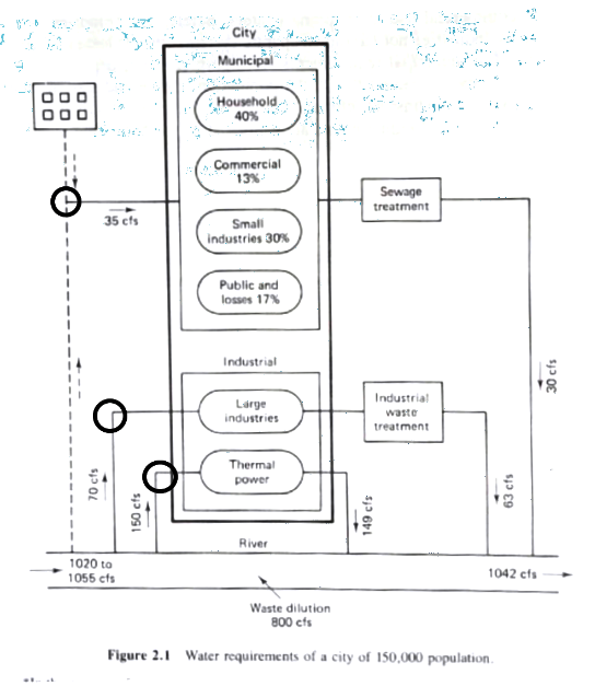
Categories of Requirements#
Municipal Requirements (Drinking Water Supply)
Large Industrial Requirements (Potable and Non-Potable)
Waste Assimilation Requirements
Municipal Requirements#
A relatively simple relationship establishes municipal requirements:
Where:
\(V_{req}\) is the volume required,
\(P_{t}\) is the population at some moment,
\(U_{per person}\) is the per person usage.
Thus the two components required to estimate demand is how many people have to be supplied, and how much each person uses.
Notice time is in the relationship. Conservation practices can influence \(U\), and growth or decline in \(P\) can also influence the volume required.
An alternative form is:
Where:
\( V \): Volume
\( P \): Population
\( \frac{V}{P} \): Volume per person
Population Forecasting#
Population forecasting uses demographic data and statistical methods to predict future water demand. This involves short-term projections for operational planning and long-term forecasts for capital investment.
Note
Population forecasting is usually outside realm of engineers; they can surely handle the arithmetic, but converting census estimates, and economic development incentives is beyond most engineers’ experiences. We can make provisional estimates for feasibility, then bring in profe$$ionals for the complete analysis.
For instance …
Consider a rapidly growing suburban area; engineers use census data and economic trends to estimate population growth. A 10-year geometric growth model predicts a 5% annual increase, helping to size reservoirs and booster stations.
Ensures infrastructure scalability for anticipated demand.
Helps in planning phased investments to avoid over- or under-building.
Graphical Methods#
Graphical methods use historical data to predict short-term demand trends, while mathematical models like geometric and arithmetic growth provide precise forecasts.
For instance …
A community uses geometric growth formulas to project a 3% annual increase in demand, enabling the timely upgrade of pipelines and treatment facilities.
Facilitates proactive infrastructure development.
Offers tools for scenario analysis and planning.
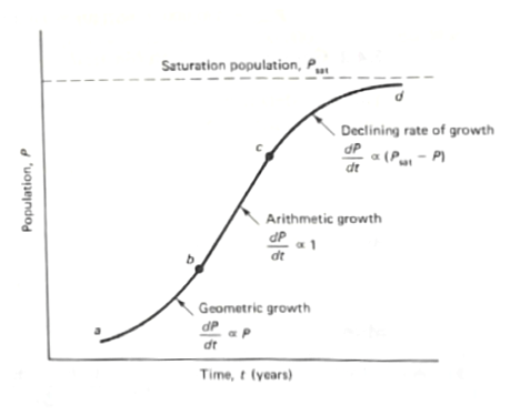
Recent history is used to determine where the target population is on the growth curve
Short-term forecasting includes:
Declining growth
Arithmetic growth
Geometric growth
Note
The curve above is identical in structure to resource capacity limited growth that you learned in Environmental Engineering (CE 3309). Examples that will follow such a curve are yeast cells in a sugar rich environment. Dextrose (glucose) is a simple sugar and is the primary energy source for yeast. It is readily taken up by yeast cells and metabolized through glycolysis, followed by either fermentation (anaerobic conditions) or respiration (aerobic conditions). In aerobic conditions the yeast cells will multiply until nearly all the dextrose is used, then the growth rate declines dramatically. The asymptote is determined to some extent by the amount of sugar originally present.
An alternative to actually drawing curves (although quite useful) is to determine the portion of interest on the curve and perform the arithmetic.
Mathematical Methods#
Geometric Growth: \( P_2 = P_1 \cdot e^{K_P (t_2 - t_1)} \)
\( K_P \): Exponential growth constant (units of recipricol time)
Arithmetic Growth: \( P_2 = P_1 + K_A (t_2 - t_1) \)
\( K_A \): Slope of the growth curve (units of recipricol time)
Declining Growth: \( P_2 = P_1 + (P_{sat} - P_1) \cdot (1 - e^{-K_D (t_2 - t_1)}) \)
\( K_D \): Declining rate constant (units of recipricol time)
Longer-Term Forecasting#
Long-term forecasting integrates demographic, economic, and environmental factors to project water demand decades into the future. This ensures sustainability and adaptability to changing conditions.
For instance …
Using population dynamics models, a city predicts that growth will stabilize after reaching 500,000 residents, guiding phased expansions of water treatment facilities.
Supports strategic decision-making for multi-decade investments.
Ensures systems are designed for long-term efficiency and sustainability.
Comparison Forecasting:#
Projects growth by comparing with geographically similar areas.
Ratio Method (Transposition):
Ratio: \( P_t = P_0 \cdot \frac{P'_t}{P'_0} \)
Where:
\( P_t \): Future population of the target area
\( P_0 \): Current population of the target area
\( P'_t \): Future population of the reference area
\( P'_0 \): Current population of the reference area
Example: If a nearby city with similar characteristics has shown consistent growth, its population ratios can help estimate the target area’s growth.
Correlation Method:
Uses statistical techniques, such as ordinary least squares (OLS), to fit a predictive equation.
Formula:
Correlation: \( P_t = a \cdot P'_t + b \) Where:
\( P_t \): Target area’s population
\( P'_t \): Reference area’s population
\( a, b \): Coefficients derived from historical data
Example: This method is particularly useful when multiple reference areas are available for comparison.
Component Techniques#
Component-based forecasting divides population dynamics into smaller measurable parts to understand the influences of births, deaths, and migration.
Births and Deaths:
Birth rate (B) and death rate (D) determine the natural increase or decrease in population.
Formula: \( P_t = P_0 + (B - D) \cdot \Delta t \)
Net Migration (M):
Accounts for people moving in or out of the area.
Formula: \( P_t = P_0 + (B - D \pm M) \cdot \Delta t \) Where:
\( M \): Net migration rate
\( \Delta t \): Time interval in years
Composite Models:
Combine multiple demographic factors (e.g., age distribution, economic conditions).
These models require significant data and computational resources but provide more accurate predictions.
Advantages of Longer-Term Forecasting#
Provides a detailed understanding of population trends.
Helps design infrastructure that meets future needs.
Incorporates economic and social factors for robust predictions.
Note
Long-term forcasting using population dynamics models is a specalist sport. In the 1980’s the solutions to the dynamic systems were by means of Routh Arrays.
The Routh Array is a mathematical tool used in control theory and differential equations to determine the stability of a system by analyzing the characteristic equation of a linear system. In the context of population dynamics models, it can be adapted to assess the stability of equilibrium points in systems governed by differential equations.
Application in Population Dynamics
Population dynamics models often involve differential equations describing the growth or decline of a population. Stability analysis determines whether the population will converge to an equilibrium (e.g., carrying capacity) or diverge (e.g., unbounded growth or extinction).
The Routh Array helps in this analysis by examining the characteristic equation derived from the linearized system of differential equations around an equilibrium point. The characteristic equation typically takes the form:
where \(s\) represents the eigenvalues, and \(a_i\) are coefficients related to the model’s parameters. (You did similar work with Lagrangian polynomials in Engineering Mathematics)
Steps in Using the Routh Array:
Construct the Characteristic Polynomial: Derive it from the population model’s linearized system.
Build the Routh Array: Organize the coefficients of the polynomial into a tabular form. Populate the rows of the array using a recursive formula derived from the coefficients.
Determine Stability:
Check the signs of the first column of the array.
If all entries in the first column are positive, the system is stable (all roots have negative real parts).
Any sign change indicates potential instability (roots with positive real parts).
Advantages:
Efficient Stability Check: The Routh Array provides stability information without explicitly solving for eigenvalues.
Insightful for Complex Models: Useful for models with higher-order dynamics where solving characteristic equations is challenging.
Example in Population Dynamics
Consider a population model with logistic growth and additional dynamics, leading to a characteristic equation like:
Using the Routh Array, we can determine whether small perturbations around the equilibrium will return to stability or diverge. Limitations
Applicable only to linearized models (near equilibrium points).
Requires the system’s differential equations to be representable in polynomial form.
This method provides a systematic way to analyze stability, making it a valuable tool in theoretical studies of population dynamics and their control mechanisms.
Today (2023) we would simply build a numerical model of the dynamic system, and perturb the model and see how it responds. In the 1980’s computers were not readily available, so mathematicians invented these clever techniques.
Water Usage#
Water usage metrics categorize demand into residential, commercial, industrial, and agricultural sectors. Average daily use and peak variations guide system component design.
For instance …
An industrial zone requires 35,000 gallons per ton for steel production, creating a high peak demand. Designers ensure the system supports this load without affecting residential supply.
Differentiates between continuous and peak demands for better resource allocation.
Informs emergency preparedness, such as fire demand capabilities.
Components#
Average Daily Demand
Hourly Variation
Fire Demand
Per Capita Usage#
Design life varies by system component.
Maintenance and replacement must account for component failures within the overall design life.
Average Daily Demand (ADD)#
Description:
Average Daily Demand (ADD) refers to the average volume of water required by a system over a 24-hour period, typically measured in gallons per day (GPD) or cubic meters per day (m³/day). It serves as a baseline for designing water systems, ensuring that infrastructure components like pipes, pumps, and storage facilities are adequately sized to meet typical daily needs.
Significance in Water System Design:
Baseline Capacity: Determines the system’s normal operating requirements.
Foundation for Variability Analysis: Serves as the basis for calculating peak demands (e.g., maximum daily demand, peak hourly demand).
Resource Planning: Helps in assessing long-term supply adequacy and operational costs.
Components of Average Daily Demand:
Residential Demand: Includes indoor uses like drinking, cooking, and bathing, as well as outdoor uses like irrigation.
Commercial Demand: Accounts for hotels, offices, and retail spaces, which often have predictable but distinct patterns.
Industrial Demand: Includes water-intensive processes like cooling, fabrication, or cleaning.
Institutional Demand: Hospitals, schools, and other facilities that cater to public needs.
Public Uses: Firefighting, street cleaning, and park irrigation.
Estimation Techniques for Average Daily Demand#
Below are common methods and tools for estimating ADD, along with a brief description of their applications:
Per Capita Consumption Method:
Description: Estimates based on the average water usage per person in the service area.
Formula:
\[ \text{ADD} = P \times U \]Where:
\( P \): Population in the service area.
\( U \): Per capita usage (gallons/person/day or liters/person/day).
Application: Suitable for municipal systems with population and usage statistics.
Historical Records:
Description: Uses historical water usage data to compute the average over a specific period.
Application: Best for established systems with reliable metering data.
Land Use Method:
Description: Estimates demand based on the type and size of land use (e.g., residential, commercial, industrial).
Application: Useful in urban planning where land use zoning is known.
Regression Models:
Description: Statistical models that correlate water demand with variables such as temperature, population, and economic activity.
Application: Ideal for analyzing demand influenced by multiple factors.
Design Standards and Guidelines:
Description: Use of standardized values from codes or guidelines, such as the Uniform Plumbing Code or American Water Works Association (AWWA) standards.
Application: Preliminary designs where specific local data is unavailable.
USGS Circular 1200:
Description: Provides maps and tables for regional water usage estimates based on past studies.
Application: Useful for broad regional studies or areas lacking metering infrastructure.
Water Balance Approach:
Description: Computes demand as the difference between total supply and losses (e.g., unaccounted-for water, leaks).
Application: Systems requiring loss quantification.
Benchmarking with Similar Communities:
Description: Uses data from demographically and geographically similar communities to estimate ADD.
Application: Helpful for new or rapidly developing areas.
Usage Monitoring and Surveys:
Description: Direct measurements from flow meters or household surveys to estimate individual and community usage.
Application: Best for targeted studies or refining existing estimates.
Illustrative Example:
A city with a population of 50,000 and an average per capita usage of 120 gallons/day would have:
This baseline can be further analyzed to determine infrastructure requirements for peak flows and storage.
Estimation Tools#
USGS Circular 1200: Maps and tables for gross estimates. (about 30 years old at time of this writing, undoubtably more recent data are available)
Approximations: Preliminary designs.
Per-Connection Calculations: Based on flow rates and plumbing capacity.
Usage Variation#
Understanding seasonal, daily, and event-driven variations ensures the system can handle peak and low-flow conditions efficiently.
For instance …
A city’s water usage spikes by 50% during a summer festival. Designers incorporate additional storage to buffer demand and avoid service interruptions.
Balances supply and demand across varying conditions.
Enhances system resilience to extreme usage scenarios.
Seasonal, daily, and special events (e.g., Super Bowl halftime).
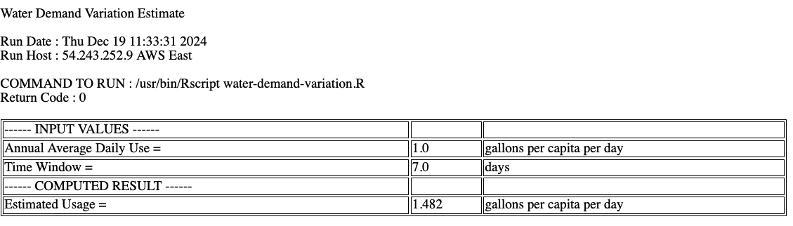
Rule-of-thumb estimate for usage variation (Goodrich, R.O. ; Gupta pp. 14-15 Eqn 1.17):
\[ \%U = \frac{180\%}{T^{0.1}} \]\( T \): Duration in days
Water Demand Variation Tool (Online Calculator that implements the above expression, with some input guidance)
#### Python Template for Estimation
import math

def usage_multiplier(duration_days):
    """Calculate usage multiplier U based on duration."""
    if duration_days <= 0:
        raise ValueError("Duration must be greater than 0.")
    U = 1.80 / (duration_days ** 0.1)
    return U

# Example usage
duration = 7  # duration in days
U = usage_multiplier(duration)
print(f"Usage multiplier U for {duration} days: {U:.2f} gallons per capita per day")
Usage multiplier U for 7 days: 1.48 gallons per capita per day
Fire Demand#
Fire demand calculations ensure the system can supply high water flow rates during emergencies. This involves considering population size, distribution, and fire department needs.
For instance …
A town with 25,000 residents calculates a fire flow demand of 19,125 GPM using population-based formulas. Hydrants and pump stations are strategically placed to meet this requirement.
Ensures public safety by supporting firefighting efforts.
Informs pipe diameter selection and pressure zone design.
Important considerations is that there are anticipated to be high withdrawal rates required during emergencies.
Fire flow calculation (cite source):
- \[ Q_{fire,GPM} = 1020 \cdot P \cdot (1 - 0.01P) \]
\( P \): Population in thousands
import math

def fire_demand(population_thousands):
    """Calculate fire flow demand based on population."""
    if population_thousands <= 0:
        raise ValueError("Population must be greater than 0.")
    Q_fire = 1020 * population_thousands * (1 - 0.01 * population_thousands)
    return Q_fire

# Example usage
population = 25  # Population in thousands
Q_fire = fire_demand(population)
print(f"Fire flow demand for a population of {population}k: {Q_fire:.2f} GPM")
Fire flow demand for a population of 25k: 19125.00 GPM
Industrial Demand#
Industrial and irrigation demands are tailored to specific applications, from cooling water in thermal plants to crop irrigation. These uses often have unique temporal and spatial characteristics.
For instance …
A petroleum refinery needs 770 gallons per barrel processed. Engineers design an independent supply line to prevent disruptions to the municipal system.
Promotes specialized designs for industrial zones.
Reduces strain on municipal supplies by segregating non-residential demands.
Typically; self-supply for large industries or community-supplied estimates based on usage rates:
Thermal Power: 80 gal/kWh
Steel Production: 35,000 gal/ton
Petroleum Refining: 770 gal/barrel
Industrial users pay different negotiated rates than most other users, usually secured by long-term contract or lease arrangements.
Waste Assimilation Demand#
Waste assimilation demand refers to the capacity of natural water bodies to dilute treated wastewater while maintaining environmental quality standards.
For instance …
A river with a flow of 40 MGD and a 60% treatment efficiency requires careful management to avoid exceeding assimilative capacity. Modeling tools like TMDL (Total Maximum Daily Load) ensure compliance.
Aligns wastewater discharge rates with treatment plant capabilities.
Supports regulatory compliance and environmental conservation.
Typically estimated using methods like TMDL or DO Sag (modeling)
Preliminary values (Gupta pp. 19-22): $\( Q_W = \frac{Q_S}{40 - 0.38 \cdot \%T} \)$
import math

def wasteflow(Q_stream,treatment):
    """Calculate waste flow demand based on source flow and treatment fraction."""
    if treatment <= 0:
        raise ValueError("treatment percent be greater than 0.")
    Q_waste = Q_stream / (40 - 0.38 * treatment)
    return Q_waste

# Example usage
Q_stream = 40  # stream flow in MGD
treatment = 60 # treatment percentage
Q_waste = wasteflow(Q_stream,treatment)
print(f"Receiving Stream Flow before Discharge {Q_stream:.2f} MGD")
print(f"Treated Sewage Assimilative Capacity {treatment}%: {Q_waste:.2f} MGD")
print(f"Total Stream Flow after Discharge {Q_waste+Q_stream:.2f} MGD")
Receiving Stream Flow before Discharge 40.00 MGD
Treated Sewage Assimilative Capacity 60%: 2.33 MGD
Total Stream Flow after Discharge 42.33 MGD
Irrigation and Other Demands#
Categories#
Irrigation: Biomass, evapotranspiration, and losses.
Other Uses:
Hydropower: Run-of-river or storage release.
Navigation: River regulation or artificial canals.