Download this file as a Jupyter Notebook@ http://54.243.252.9/ce-3372-webroot/2-Exercises/ES9/ES9.ipynb
ES-9 Solution Sketch
Copyright © 2022 Theodore G. Cleveland
Purpose:
Construct a design storm hyetograph
Problem Statement
Assume that Somewhere USA is to be located in Harris County.
Part 1 (Check Syllabus/BB for Due Date)
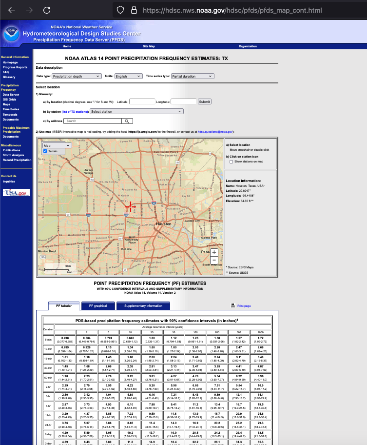
- Using the NOAA-PFDS estimate the rainfall depth for a 10-year, 6-hour storm in Harris county.
- Using the SCS Tabulation or Texas Empirical Hyetographs, construct from the 10-year, 6-hour storm a design hyetograph at 15 minute intervals.

| Figure 1. Screen capture PFDS for Harris Co. Interrogation |
|---|
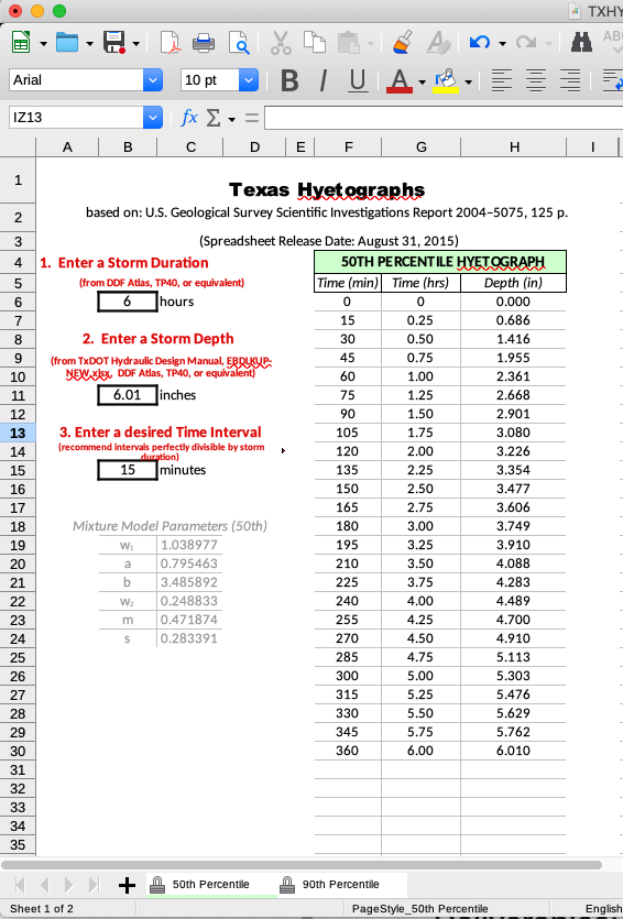
From the figure, a 10-yr, 6-hr storm is 6.10 inches of depth. Next using the Texas Empirical Hyetograph we produce the following hyetograph (using the median hyetograph)

| Figure 2. Screen capture Texas Hyetograph Tool |
|---|
The actual numbers are captured below:
import pandas
hyetograph = pandas.DataFrame([[0,0,0.000],
[15,0.25,0.686],
[30,0.50,1.416],
[45,0.75,1.955],
[60,1.00,2.361],
[75,1.25,2.668],
[90,1.50,2.901],
[105,1.75,3.080],
[120,2.00,3.226],
[135,2.25,3.354],
[150,2.50,3.477],
[165,2.75,3.606],
[180,3.00,3.749],
[195,3.25,3.910],
[210,3.50,4.088],
[225,3.75,4.283],
[240,4.00,4.489],
[255,4.25,4.700],
[270,4.50,4.910],
[285,4.75,5.113],
[300,5.00,5.303],
[315,5.25,5.476],
[330,5.50,5.629],
[345,5.75,5.762],
[360,6.00,6.010]])
hyetograph.columns =["minutes","hours","acc_depth_inches"]
hyetograph.head()
# plot the hyetograph as per ENGR 1330
from matplotlib import pyplot as plt
mydata = plt.figure(figsize = (8,6)) # build a drawing canvass from figure class; aspect ratio 4x3
plt.plot(hyetograph["hours"],hyetograph["acc_depth_inches"], c='red', marker='o',linewidth=1) # basic line plot
plt.xlabel('Elapsed Time (hours)') # label the x-axis
plt.ylabel('Accumulated Rainfall Depth (inches)') # label the y-axis, notice the LaTex markup
#plt.legend(['series1','series2...']) # legend for each series
plt.title('Somewhere USA Design Storm') # make a plot title
plt.grid() # display a grid
plt.show() # display the plot
# prep the data for cut-and-paste into SWMM
print(hyetograph[["hours","acc_depth_inches"]].to_string(index=False))
Part 2 (Check Syllabus/BB for Due Date)
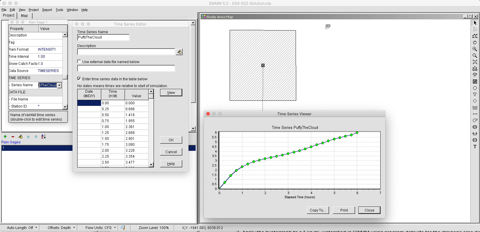
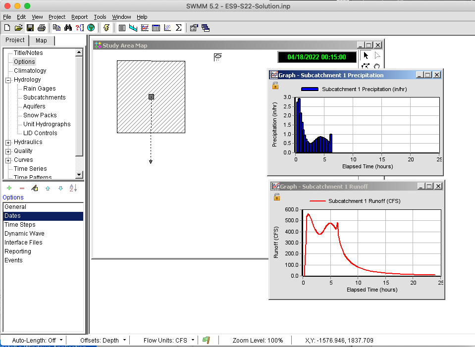
- Apply the hyetograph to a 1 sq.mi. watershed in SWMM using program defaults for the drainage area description (except set the length to 5280 ft.), use the CN runoff generation model in SWMM with CN=98. Simulate 24 hours of runoff with reporting every 15 minutes.

| Figure 3. Screen capture SWMM set-up raingage (named PuffyTheCloud) |
|---|

|Figure 4. Screen capture SWMM run using CN=98, and supplied hyetograph| |---|
Deliverables:
A brief report with your solution, showing the rainfall depth(s), hyetograph (on 15-minute intervals) for Part 1 and the SWMM generated hydrograph for Part 2.
A screen capture of the SWMM output is sufficient for Part 2 Do not submit a SWMM output file
References
- NOAA Precipitation-Frequency Data Server https://hdsc.nws.noaa.gov/hdsc/pfds/
- Intensity Interpolater (for use with PFDS results) for non-tabulated durations. http://54.243.252.9/toolbox/ordinarytools/IntensityInterpolate/IntensityInterpolate.html 2.Williams-Sether, T., Asquith, W.H., Thompson, D.B., Cleveland, T.G., and X. Fang. 2004. Empirical, Dimensionless, Cumulative-Rainfall Hyetographs for Texas. U.S.Geological Survey Scientific Investigations Report 2004-5075, 138p. https://75.3.84.227/documents/about-me/MyWebPapers/project_reports/SIR_2004_5075/sir2004-5075.pdf
- Neale, C.M., Tay, C.C., Herrmann, G.R., and Cleveland, T.G. 2015. "TXHYETO.XLS a tool to facilitate use of Texas-Specific Hyetographs for design storm modeling." Proceedings of ASCE World Environmental and Water Resources Congress, ASCE-EWRI, Austin, TX. May 17-21, 2015. pp. 241-254.https://75.3.84.227/documents/about-me/MyWebPapers/conference_papers/2015_ASCE_CAROLINE/
- TXHYETO (spreadsheet and training video for using Texas empirical hyetographs)http://54.243.252.9/toolbox/hydrology/EBDLKUP-2015-DISTRIBUTE/
- Rossman, L.A., 2010 STORM WATER MANAGEMENT MODEL USER’S MANUAL Version 5.0, Technical Report EPA/600/R-05/040,U.S. Environmental Protection Agency, National Risk Management Research Laboratory Cincinnati, OH 45268. http://54.243.252.9/ce-3372-webroot/3-Readings/epaswmm5_user_manual/P100ERK4.pdf
- Rossman, L.A., 2006 STORM WATER MANAGEMENT MODEL QUALITY ASSURANCE REPORT: Dynamic Wave Flow Routing, Technical Report EPA/600/R-06/297,U.S. Environmental Protection Agency, National Risk Management Research Laboratory Cincinnati, OH 45268. http://54.243.252.9/ce-3372-webroot/3-Readings/epaswmm5_qa/SWMM5_QA.pdf
- Gironás, J., Roesner, L.A., Davis, J. 2009 STORM WATER MANAGEMENT MODEL APPLICATIONS MANUAL , Technical Report EPA/600/R-09/000,U.S. Environmental Protection Agency, National Risk Management Research Laboratory Cincinnati, OH 45268. http://54.243.252.9/ce-3372-webroot/3-Readings/epaswmm5_user_manual/P100ERK4.pdf
