# Environment Check -- Deactivate on a working host
import sys
print(sys.executable)
print(sys.version)
print(sys.version_info)
Application of Linear Systems Analysis
A typical static truss analysis problem goes like
"The figure below is a simply supported, statically determinate truss with pin connections (zero moment transfer connections). Find the forces in each member for the loading shown."
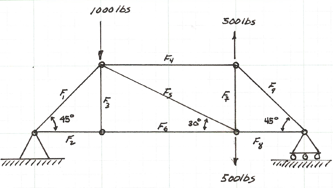
This notebook will illustrate how to leverage our linear systems solver(s) to analyze the truss. The approach uses concepts from statics and computational thinking.
From statics
1) method of joints (for reactions and internal forcez)
2) direction cosines
From computational thinking
1) read input file
2) construct linear system \textbf{Ax=b}; solve for \textbf{x}
3) report results
Before even contemplating writing/using a program we need to build a mathematical model of the truss and assemble the system of linear equations that result from the model.
So the first step is to sketch a free-body-diagram as below and build a node naming convention and force names.
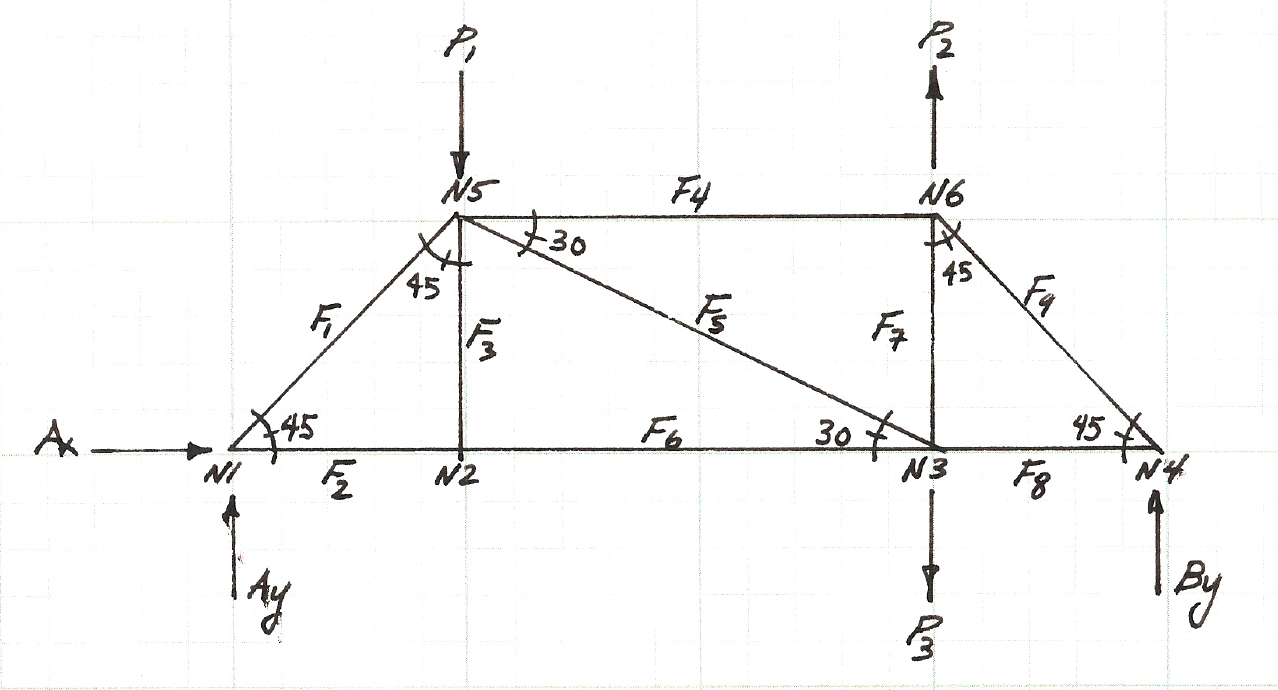
Next we will write the force balance for each of the six nodes ($N1$-$N6$), which will produce a total of 12 equations in the 12 unknowns (the 9 member forces, and 3 reactions).
The figure below is the force balance for node $N1$, the two force equations (for the horizontal, $x$, direction and the vertical, $y$, direction) are listed below the figure.
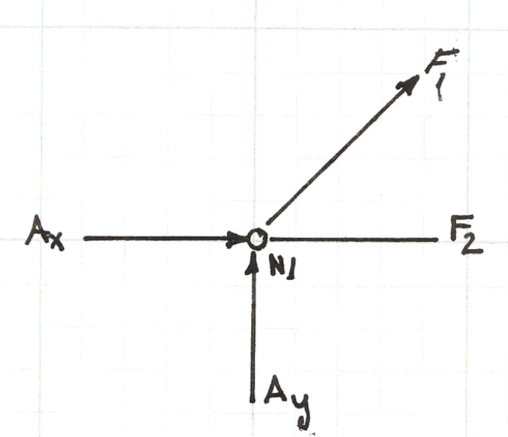
The equation above is the force balance equation pair for the node. The $x$ component equation will later be named $N1_x$ to indicate it arises from Node 1, $x$ component equation. A similar notation convention will also be adopted for the $y$ component equation. There will be an equation pair for each node.
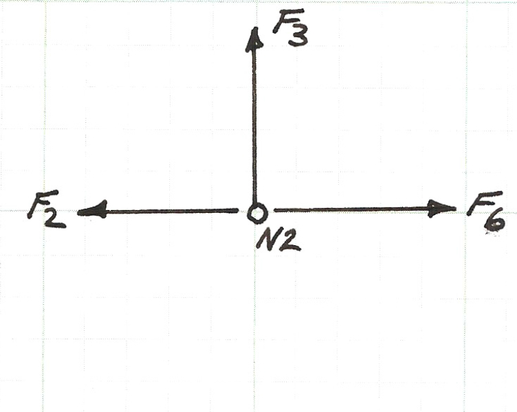
Below is a sketch of the force balance for node $N2$, the two force equations (for the horizontal, $x$, direction and the vertical, $y$, direction) are listed below the figure.
Below is a sketch of the force balance for node $N3$, the two force equations (for the horizontal, $x$, direction and the vertical, $y$, direction) are listed below the figure.
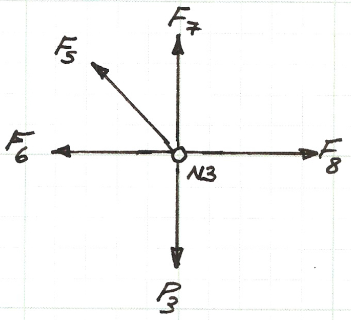
Above is the force balance equation pair for node $N3$.
Below is a sketch of the force balance for node $N4$, the two force equations (for the horizontal, $x$, direction and the vertical, $y$, direction) are listed below the figure.
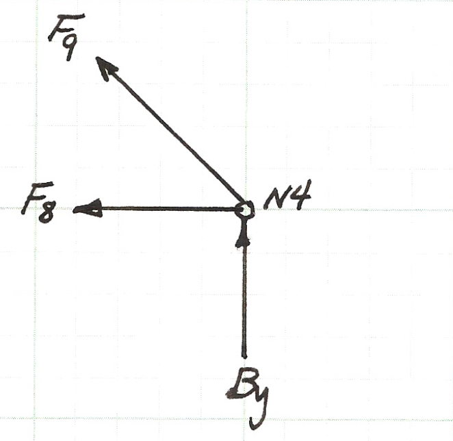
Above is the force balance equation pair for node $N4$.
Below is a sketch of the force balance for node $N5$, the two force equations (for the horizontal, $x$, direction and the vertical, $y$, direction) are listed below the figure.
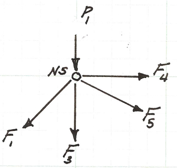
Above is the force balance equation pair for node $N5$.
Below is a sketch of the force balance for node $N6$, the two force equations (for the horizontal, $x$, direction and the vertical, $y$, direction) are listed below the figure.
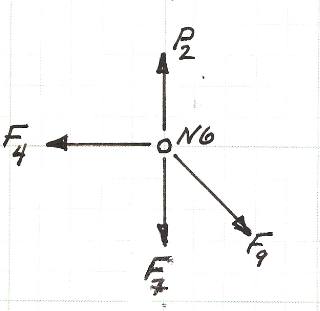
Above is the force balance equation pair for node $N6$.
The next step is to gather the equation pairs into a system of linear equations.
We will move the known loads to the right hand side and essentially construct the matrix equation $\mathbf{A}\mathbf{x} = \mathbf{b}$.
The system below is a matrix representation of the equation pairs with the forces moved to the right hand side $\mathbf{b} = RHS$.
\begin{gather} \begin{pmatrix} ~ & F_1 & F_2 & F_3 & F_4 & F_5 & F_6 & F_7 & F_8 & F_9 & A_x & A_y & B_y & | & RHS\\ \hline N1_x & 0.707 & 1 & 0 & 0 & 0 & 0 & 0 & 0 & 0 & 1 & 0 & 0 & | & 0\\ N1_y & 0.707 & 0 & 0 & 0 & 0 & 0 & 0 & 0 & 0 & 0 & 1 & 0 & | & 0\\ N2_x & 0 & -1 & 0 & 0 & 0 & 1 & 0 & 0 & 0 & 0 & 0 & 0 & | & 0\\ N2_y & 0 & 0 & 1 & 0 & 0 & 0 & 0 & 0 & 0 & 0 & 0 & 0 & | & 0\\ N3_x & 0 & 0 & 0 & 0 & -0.866 & -1 & 0 & 1 & 0 & 0 & 0 & 0 & | & 0\\ N3_y & 0 & 0 & 0 & 0 & 0.5 & 0 & 1 & 0 & 0 & 0 & 0 & 0 & | & P_3\\ N4_x & 0 & 0 & 0 & 0 & 0 & 0 & 0 & -1 & -0.707 & 0 & 0 & 0 & | & 0\\ N4_y & 0 & 0 & 0 & 0 & 0 & 0 & 0 & 0 & 0.707 & 0 & 0 & 0 & | & 0\\ N5_x & -0.707 & 0 & 0 & 1 & 0.866 & 0 & 0 & 0 & 0 & 0 & 0 & 0 & | & 0\\ N5_y & -0.707 & 0 & -1 & 0 & -0.5 & 0 & 0 & 0 & 0 & 0 & 0 & 0 & | & P_1\\ N6_x & 0 & 0 & 0 & -1 & 0 & 0 & 0 & 0 & 0.707 & 0 & 0 & 0 & | & 0\\ N6_y & 0 & 0 & 0 & 0 & 0 & 0 & -1 & 0 & -0.707 & 0 & 0 & 0 & | & -P_2\\ \end{pmatrix} \end{gather}In the system, the rows are labeled on the left-most column with their node-related equation name.
Thus each row of the matrix corresponds to an equation derived from a node.
The columns are labeled with their respective unknown force (except the last column, which represents the right-hand-side of the system of linear equations).
Thus the coefficient in each column corresponds to a force in each node equation.
The sign of the coefficient refers to the assumed direction the force acts.
In the analysis all the members were assumed to be in tension (except for the reaction forces).
If a coefficient has a value of zero in a particular row, then that force does no act at the node to which the row corresponds.
From this representation the transition to the formal vector-matrix representation is straightforward.
The various matrices above are entere into text files named A.txt and B.txt, we can examine the file contents using the host OS as below
# list contents of the A matrix, uses call to OS host
!(cat A.txt)
# list contents of RHS or b vector
!(cat B.txt)
Now we use our solver tools, here I have not doen much on tidy output, thats left for the reader.
# Linear System Solver

from LinearSolverPivot import linearsolver

amatrix = [] # null list to store matrix reads
bvector = []
rowNumA = 0
colNumA = 0
rowNumB = 0
afile = open("A.txt","r")  # connect and read file for MATRIX A
for line in afile:
    amatrix.append([float(n) for n in line.strip().split()])
    rowNumA += 1
afile.close() # Disconnect the file
colNumA = len(amatrix[0])
afile = open("B.txt","r")  # connect and read file for MATRIX B
for line in afile:
    bvector.append(float(line))  # vector read different -- just float the line
    rowNumB += 1
afile.close() # Disconnect the file
#print (bvector)
if rowNumA != rowNumB:   # check the arrays
    print ("row ranks not same -- aborting now")
    quit()
else:
    print ("row ranks same -- continuing operation")
# print all columns each row
cmatrix = [[0 for j in range(colNumA)]for i in range(rowNumA)]
dmatrix = [[0 for j in range(colNumA)]for i in range(rowNumA)]
xvector = [0 for i in range(rowNumA)]
dvector = [0 for i in range(rowNumA)]
for i in range(0,rowNumA,1):
    print (amatrix[i][0:colNumA], bvector[i])
print ("-----------------------------")
# copy amatrix into cmatrix
cmatrix = [[amatrix[i][j] for j in range(colNumA)]for i in range(rowNumA)]
dmatrix = [[amatrix[i][j] for j in range(colNumA)]for i in range(rowNumA)]
dvector = [bvector[i] for i in range(rowNumA)]
dvector = linearsolver(amatrix,bvector)
for i in range(0,rowNumA,1):
    print (dvector[i])
print ("-----------------------------")
References
Overland, B. (2018). Python Without Fear. Addison-Wesley ISBN 978-0-13-468747-6.
Grus, Joel (2015). Data Science from Scratch: First Principles with Python O’Reilly Media. Kindle Edition.
Precord, C. (2010) wxPython 2.8 Application Development Cookbook Packt Publishing Ltd. Birmingham , B27 6PA, UK ISBN 978-1-849511-78-0.