Laboratory 20: "Confidence in Linear Regression" or "The Exclusive Guide to Trial by Combat in Westeros"
# Preamble script block to identify host, user, and kernel
import sys
! hostname
! whoami
print(sys.executable)
print(sys.version)
print(sys.version_info)

Last week, we talked about linear regression ...

- What is linear regression?
a basic predictive analytics technique that uses historical data to predict an output variable. - Why do we need linear regression?
To explore the relationship between predictor and output variables and predict the output variable based on known values of predictors.
- How does linear regression work?
To estimate Y using linear regression, we assume the equation: 𝑌𝑒=β𝑋+α
Our goal is to find statistically significant values of the parameters α and β that minimise the difference between Y and Yₑ. If we are able to determine the optimum values of these two parameters, then we will have the line of best fit that we can use to predict the values of Y, given the value of X. - How to estimate the coefficients? We have used "Ordinary Least Squares (OLS)" and "Maximum Likelihood Estimation (MLE)" methods. We can get formulas for the slope and intercept of the line of best fit from each method. Once we have the equation of the line of best fit, we can use it to fit a line and assess the quality of fit as well as predicting.
- How to assess the fit? We have used graphs and visual assessments to describe the fits, identify regions with more and less errors, and decide whether the fit is trustworthy or not.
We also use "Goodness-of-Fit (GOF)" metrics to describe the errors and performance of the linear models.
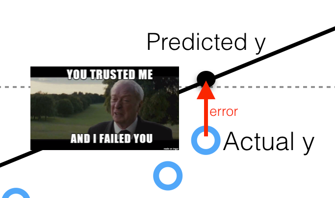
- How confident are we with a prediction? By definition, the prediction of a linear regression model is an estimate or an approximation and contains some uncertainty. The uncertainty comes from the errors in the model itself and noise in the input data. The model is an approximation of the relationship between the input variables and the output variables. The model error can be decomposed into three sources of error: the variance of the model, the bias of the model, and the variance of the irreducible error (the noise) in the data.
Error(Model) = Variance(Model) + Bias(Model) + Variance(Irreducible Error)
That time in Westeros...
Before going any further, let's assume that you were arrested by the king's guard as you were minding your business in the streets of King's Landing for the crime of planning for the murder of King Joffrey Baratheon. As much as you hate King Joffrey you had no plans for killing him but no one believes you. In the absence of witnesses or a confession, you demand trial by combat.

But they inform you that the Germanic law to settle accusations is no longer used and it has been replaced with a new method. You get to choose a bowman. That bowman will make 3 shots for you. And if he hits the bullseye you will walk a free man. Otherwise, you will be hanged.

You have two options. The first bowman is Horace. He is known as one of the greatest target archers of all time. He is old though and due to lack of an efficient social security system in Westeros, he has to work as a hired bowman for the high court to earn a living. You ask around and you hear that he still can shoot a bullseye but as his hands shake, he sometimes misses by a lot. The second archer is Daryl. He is also a wellknown archer but unfortunately he has a drinking problem. You have understood that there has been cases that he has shot the bullseye in all of his three shots and there has been cases that he has completely missed the bullseye. The thing about him is that his three shots are always very close together. Now, you get to pick. Between Horace and Daryl, who would you choose to shoot for your freedom?
- Bias, Variance, and the bowman dilemma!
We used the example above to give you an initial understanding of bias and variance and their impact on a model's performance. Given this is a complicated and yet important aspect of data modeling and machine learning, without getting into too much detail, we will discuss these concepts. Bias reflects how close the functional form of the model can get to the true relationship between the predictors and the outcome. Variance refers to the amount by which [the model] would change if we estimated it using a different training data set.
Looking at the picture above, Horace was an archer with high variance and low bias, while Daryl had high bias and low variability. In an ideal world, we want low bias and low variance which we cannot have. When there is a high bias error, it results in a very simplistic model that does not consider the variations very well. Since it does not learn the training data very well, it is called Underfitting. When the model has a high variance, it will still consider the noise as something to learn from. That is, the model learns the noise from the training data, hence when confronted with new (testing) data, it is unable to predict accurately based on it. Since in the case of high variance, the model learns too much from the training data, it is called overfitting. To summarise:
- A model with a high bias error underfits data and makes very simplistic assumptions on it
- A model with a high variance error overfits the data and learns too much from it
- A good model is where both Bias and Variance errors are balanced. The balance between the Bias error and the Variance error is the Bias-Variance Tradeoff.
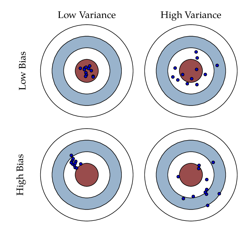
The irreducible error is the error that we can not remove with our model, or with any model. The error is caused by elements outside our control, such as statistical noise in the observations. A model with low bias and high variance predicts points that are around the center generally, but pretty far away from each other (Horace). A model with high bias and low variance is pretty far away from the bull’s eye, but since the variance is low, the predicted points are closer to each other (Daryl). Bias and Variance play an important role in deciding which predictive model to use: Something that you will definitly learn more about if you go further in the field of machine learning and predicitve models.
How can we measure bias and variance?
There are GOF metrics that can measure the bias and variance of a model: For example the Nash–Sutcliffe model efficiency coefficient and the Kling-Gupta Efficiency (KGE). The Nash–Sutcliffe efficiency is calculated as one minus the ratio of the error variance of the modeled time-series divided by the variance of the observed time-series. In the situation of a perfect model with an estimation error variance equal to zero, the resulting Nash-Sutcliffe Efficiency equals 1 (NSE = 1). KGE provides a diagnostically interesting decomposition of the Nash-Sutcliffe efficiency (and hence MSE), which facilitates the analysis of the relative importance of its different components (correlation, bias and variability).
Example 1: Let's have a look at our old good example of TV, Radio, and Newspaper advertisements and number of sales for a specific product.!
Let's say that we are interested to compare the performance of the linear models that use TV spendings and Radio spendings as their predictor variables in terms of accuracy, bias, and variability.
import numpy as np
import pandas as pd
import statistics
import scipy.stats
from matplotlib import pyplot as plt
import statsmodels.formula.api as smf
import sklearn.metrics as metrics

# Import and display first rows of the advertising dataset
df = pd.read_csv('advertising.csv')
tv = np.array(df['TV'])
radio = np.array(df['Radio'])
newspaper = np.array(df['Newspaper'])
sales = np.array(df['Sales'])
# Initialise and fit linear regression model using `statsmodels`
# TV Spending as predictor
model_tv = smf.ols('Sales ~ TV', data=df)
model_tv = model_tv.fit()
TV_pred = model_tv.predict()
# Radio Spending as predictor
model_rd = smf.ols('Sales ~ Radio', data=df)
model_rd = model_rd.fit()
RD_pred = model_rd.predict()
print("RMSE for TV ad spendings as predictor is ",np.sqrt(metrics.mean_squared_error(sales, TV_pred)))
print("RMSE for Radio ad spendings as predictor is ",np.sqrt(metrics.mean_squared_error(sales, RD_pred)))
print("R2 for TV ad spendings as predictor is ",metrics.r2_score(sales, TV_pred))
print("R2 for Radio ad spendings as predictor is ",metrics.r2_score(sales, RD_pred))
from scipy.stats import pearsonr
tv_r = pearsonr(TV_pred, sales)
rd_r = pearsonr(RD_pred, sales)

print("Pearson's r for TV ad spendings as predictor is ",tv_r[0])
print("Pearson's for Radio ad spendings as predictor is ",rd_r[0])
from hydroeval import *          #Notice this importing method
tv_nse = evaluator(nse, TV_pred, sales)
rd_nse = evaluator(nse, RD_pred, sales)

print("NSE for TV ad spendings as predictor is ",tv_nse)
print("NSE for Radio ad spendings as predictor is ",rd_nse)
tv_kge = evaluator(kgeprime, TV_pred, sales)
rd_kge = evaluator(kgeprime, RD_pred, sales)

print("KGE for TV ad spendings as predictor is ",tv_kge)
print("KGE for Radio ad spendings as predictor is ",rd_kge)
#KGE: Kling-Gupta efficiencies range from -Inf to 1. Essentially, the closer to 1, the more accurate the model is.
#r: the Pearson product-moment correlation coefficient. Ideal value is r=1
#Gamma: the ratio between the coefficient of variation (CV) of the simulated values to
       #the coefficient of variation of the observed ones. Ideal value is Gamma=1
#Beta: the ratio between the mean of the simulated values and the mean of the observed ones. Ideal value is Beta=1
How confident are we with our linear regression model?
The 95% confidence interval for the forecasted values ŷ of x is

where

This means that there is a 95% probability that the true linear regression line of the population will lie within the confidence interval of the regression line calculated from the sample data.

In the graph on the left of Figure 1, a linear regression line is calculated to fit the sample data points. The confidence interval consists of the space between the two curves (dotted lines). Thus there is a 95% probability that the true best-fit line for the population lies within the confidence interval (e.g. any of the lines in the figure on the right above).
There is also a concept called a prediction interval. Here we look at any specific value of x, x0, and find an interval around the predicted value ŷ0 for x0 such that there is a 95% probability that the real value of y (in the population) corresponding to x0 is within this interval (see the graph on the right side). The 95% prediction interval of the forecasted value ŷ0 for x0 is

where the standard error of the prediction is

For any specific value x0 the prediction interval is more meaningful than the confidence interval.

Example 2: Let's work on another familier example.
We had a table of recoded times and speeds from some experimental observations:
| Elapsed Time (s) | Speed (m/s) |
|---|---|
| 0 | 0 |
| 1.0 | 3 |
| 2.0 | 7 |
| 3.0 | 12 |
| 4.0 | 20 |
| 5.0 | 30 |
| 6.0 | 45.6 |
| 7.0 | 60.3 |
| 8.0 | 77.7 |
| 9.0 | 97.3 |
| 10.0 | 121.1 |
This time we want to explore the confidence and prediciton intervals for our linear regression model:
time = [0, 1.0, 2.0, 3.0, 4.0, 5.0, 6.0, 7.0, 8.0, 9.0, 10.0]
speed = [0, 3, 7, 12, 20, 30, 45.6, 60.3, 77.7, 97.3, 121.2]
x = np.array(time)
Y = np.array(speed)

#We already know these parameters from last week but let's assume that we don't!
# alpha = -16.78636363636364
# beta = 11.977272727272727
#Our linear model: ypred = alpha + beta * x

import statsmodels.api as sm     #needed for linear regression
from statsmodels.sandbox.regression.predstd import wls_prediction_std   #needed to get prediction interval
X = sm.add_constant(x)
re = sm.OLS(Y, X).fit()
print(re.summary())
print(re.params)
prstd, iv_l, iv_u = wls_prediction_std(re) #iv_l and iv_u give you the limits of the prediction interval for each point.
print(iv_l)
print(iv_u)
from statsmodels.stats.outliers_influence import summary_table

st, data, ss2 = summary_table(re, alpha=0.05)

fittedvalues = data[:, 2]
predict_mean_se  = data[:, 3]
predict_mean_ci_low, predict_mean_ci_upp = data[:, 4:6].T
predict_ci_low, predict_ci_upp = data[:, 6:8].T


plt.plot(x, Y, 'o')
plt.plot(x, fittedvalues, '-',color='red', lw=2)
#plt.plot(x, predict_ci_low, '--', color='green',lw=2) #Lower prediction band
#plt.plot(x, predict_ci_upp, '--', color='green',lw=2) #Upper prediction band
#plt.plot(x, predict_mean_ci_low,'--', color='orange',  lw=2) #Lower confidence band
#plt.plot(x, predict_mean_ci_upp,'--', color='orange', lw=2) #Upper confidence band
plt.show()


This notebook was inspired by several blogposts including:
- "How to Calculate the Bias-Variance Trade-off with Python" by Jason Brownlee available at* https://machinelearningmastery.com/calculate-the-bias-variance-trade-off/
- "Bias and Variance in Machine Learning – A Fantastic Guide for Beginners!" by PURVA HUILGOL available at* https://www.analyticsvidhya.com/blog/2020/08/bias-and-variance-tradeoff-machine-learning/
- "Prediction Intervals for Machine Learning" by Jason Brownlee available at* https://machinelearningmastery.com/prediction-intervals-for-machine-learning/
- "Confidence and prediction intervals for forecasted values" by Charles Zaiontz available at* https://www.real-statistics.com/regression/confidence-and-prediction-intervals/
- "3.7 OLS Prediction and Prediction Intervals" available at* http://web.vu.lt/mif/a.buteikis/wp-content/uploads/PE_Book/3-7-UnivarPredict.html
- "Using python statsmodels for OLS linear regression" available at* https://markthegraph.blogspot.com/2015/05/using-python-statsmodels-for-ols-linear.html
Here are some great reads on these topics:
- "How to Calculate the Bias-Variance Trade-off with Python" available at* https://aidevelopmenthub.com/how-to-calculate-the-bias-variance-trade-off-with-python/
- "Understanding the Bias-Variance Tradeoff" available at* http://scott.fortmann-roe.com/docs/BiasVariance.html
- "SCIKIT-LEARN : BIAS-VARIANCE TRADEOFF" available at* https://www.bogotobogo.com/python/scikit-learn/scikit_machine_learning_Bias-variance-Tradeoff.php
- "Linear Regression Confidence Intervals" available at* https://rstudio-pubs-static.s3.amazonaws.com/195401_20b3272a8bb04615ae7ee4c81d18ffb5.html
- "Prediction Interval: Simple Definition, Examples" available at* https://www.statisticshowto.com/prediction-interval/
Here are some great videos on these topics:
- "Machine Learning Fundamentals: Bias and Variance" by StatQuest with Josh Starmer available at* https://www.youtube.com/watch?v=EuBBz3bI-aA
- "Bias Variance Trade off" by The Semicolon available at* https://www.youtube.com/watch?v=lpkSGTT8uMg
- "Intervals (for the Mean Response and a Single Response) in Simple Linear Regression" by jbstatistics available at* https://www.youtube.com/watch?v=V-sReSM887I
- "Calculate Confidence and prediction intervals for a response in SLR by hand" by Katie Ann Jager available at* https://www.youtube.com/watch?v=JqObYVX1UP0