Download (right-click, save target as ...) this page as a jupyterlab notebook Lab26
Laboratory 26: Regression Models
LAST NAME, FIRST NAME
R00000000
ENGR 1330 Laboratory 26 - In Lab
Prediction Engines and Regression
The human brain is amazing and mysterious in many ways.
Have a look at these sequences.
You, with the assistance of your brain, can guess the next item in each sequence, right?
- A,B,C,D,E, __ ?
- 5,10,15,20,25, __ ?
- 2,4,8,16,32 __ ?
- 0,1,1,2,3, __ ?
- 1, 11, 21, 1211,111221, __ ?


But how does our brain do this? How do we 'guess | predict' the next step?
Is it that there is only one possible option? is it that we have the previous items? or is it the relationship between the items?
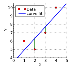
What if we have more than a single sequence? Maybe two sets of numbers? How can we predict the next "item" in a situation like that?

Blue Points? Red Line? Fit? Does it ring any bells?

Example 1 (May wish to skip to the statsmodel part below!)
The table below contains some experimental observations.
| Elapsed Time (s) | Speed (m/s) |
|---|---|
| 0 | 0 |
| 1.0 | 3 |
| 2.0 | 7 |
| 3.0 | 12 |
| 4.0 | 20 |
| 5.0 | 30 |
| 6.0 | 45.6 |
| 7.0 | 60.3 |
| 8.0 | 77.7 |
| 9.0 | 97.3 |
| 10.0 | 121.1 |
- Plot the speed vs time (speed on y-axis, time on x-axis) using a scatter plot. Use blue markers.
- Plot a red line on the scatterplot based on the linear model $f(x) = mx + b$
- By trial-and-error find values of $m$ and $b$ that provide a good visual fit (i.e. makes the red line explain the blue markers).
- Using this data model estimate the speed at $t = 15~\texttt{sec.}$

Terminology:
Linear Regression: a predictive analytics technique that uses observed data to predict an output variable.
The Predictor variable (input): the variable(s) that help predict the value of the output variable. It is commonly referred to as X.
The Output/Response variable: the variable that we want to predict. It is commonly referred to as Y.
To estimate Y using linear regression, we stipulate the model equation: $Y_e = \beta X + \alpha $,
where $Y_ₑ$ is the estimated or predicted value of Y based on our linear equation.
A meaningful goal is to find statistically significant values of the parameters $\alpha$ and $\beta$ that minimise the difference between $Y_o$ and $Y_e$.
If we are able to determine the optimum values of these two parameters, then we will have the line of best fit that we can use to predict the values of Y, given the value of X.
So, how do we estimate α and β?

We can use a method called Ordinary Least Squares (OLS).
The objective of the least squares method is to find values of $\alpha$ and $\beta$ that minimise the sum of the squared difference between $Y_o$ and $Y_e$ (distance between the linear fit and the observed points).
We will not go through the derivation here, but using calculus we can show that the values of the unknown parameters are as follows:
where $\bar X$ is the mean of $X$ values and $\bar Y$ is the mean of $Y$ values. $\beta$ is simply the covariance of $X$ and $Y$ (Cov(X, Y) divided by the variance of $X$ (Var(X)).
Covariance: In probability theory and statistics, covariance is a measure of the joint variability of two random variables. If the greater values of one variable mainly correspond with the greater values of the other variable, and the same holds for the lesser values, (i.e., the variables tend to show similar behavior), the covariance is positive. In the opposite case, when the greater values of one variable mainly correspond to the lesser values of the other, (i.e., the variables tend to show opposite behavior), the covariance is negative. The sign of the covariance therefore shows the tendency in the linear relationship between the variables. The magnitude of the covariance is not easy to interpret because it is not normalized and hence depends on the magnitudes of the variables. The normalized version of the covariance, the correlation coefficient, however, shows by its magnitude the strength of the linear relation.

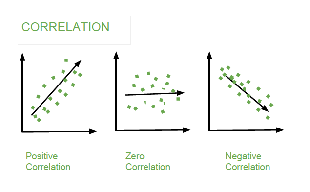
The Correlation Coefficient: Correlation coefficients are used in statistics to measure how strong a relationship is between two variables. There are several types of correlation coefficient, but the most popular is Pearson’s. Pearson’s correlation (also called Pearson’s R) is a correlation coefficient commonly used in linear regression.Correlation coefficient formulas are used to find how strong a relationship is between data. The formula for Pearson’s R:
The formulas return a value between -1 and 1, where:
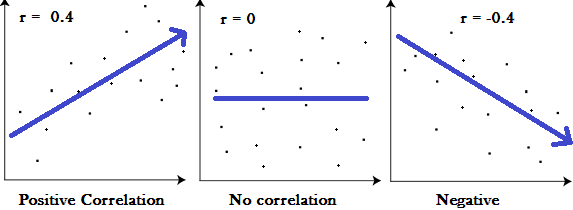
1 : A correlation coefficient of 1 means that for every positive increase in one variable, there is a positive increase of a fixed proportion in the other. For example, shoe sizes go up in (almost) perfect correlation with foot length.
-1: A correlation coefficient of -1 means that for every positive increase in one variable, there is a negative decrease of a fixed proportion in the other. For example, the amount of gas in a tank decreases in (almost) perfect correlation with speed.
0 : Zero means that for every increase, there isn’t a positive or negative increase. The two just aren’t related.
Now Let's have a look at the Example
We had a table of recorded times and speeds from some experimental observations:
| Elapsed Time (s) | Speed (m/s) |
|---|---|
| 0 | 0 |
| 1.0 | 3 |
| 2.0 | 7 |
| 3.0 | 12 |
| 4.0 | 20 |
| 5.0 | 30 |
| 6.0 | 45.6 |
| 7.0 | 60.3 |
| 8.0 | 77.7 |
| 9.0 | 97.3 |
| 10.0 | 121.1 |
First let's create a dataframe:
# Load the necessary packages
import numpy as np
import pandas as pd
import statistics
from matplotlib import pyplot as plt

# Create a dataframe:
time = [0, 1.0, 2.0, 3.0, 4.0, 5.0, 6.0, 7.0, 8.0, 9.0, 10.0]
speed = [0, 3, 7, 12, 20, 30, 45.6, 60.3, 77.7, 97.3, 121.2]
data = pd.DataFrame({'Time':time, 'Speed':speed})
data
Now, let's explore the data:
data.describe()
time_var = statistics.variance(time)
speed_var = statistics.variance(speed)

print("Variance of recorded times is ",time_var)
print("Variance of recorded times is ",speed_var)
Is there a relationship ( based on covariance, correlation) between time and speed?
# To find the covariance
data.cov()
# To find the correlation among the columns
# using pearson method
data.corr(method ='pearson')
Let's do linear regression with primitive Python:
- To estimate "y" using the OLS method, we need to calculate "xmean" and "ymean", the covariance of X and y ("xycov"), and the variance of X ("xvar") before we can determine the values for alpha and beta. In our case, X is time and y is Speed.
# Calculate the mean of X and y
xmean = np.mean(time)
ymean = np.mean(speed)

# Calculate the terms needed for the numator and denominator of beta
data['xycov'] = (data['Time'] - xmean) * (data['Speed'] - ymean)
data['xvar'] = (data['Time'] - xmean)**2

# Calculate beta and alpha
beta = data['xycov'].sum() / data['xvar'].sum()
alpha = ymean - (beta * xmean)
print(f'alpha = {alpha}')
print(f'beta = {beta}')
We now have an estimate for alpha and beta! Our model can be written as $Y_e = 11.977 X -16.786$, and we can make predictions:
X = np.array(time)

ypred = alpha + beta * X
print(ypred)
Let’s plot our prediction ypred against the actual values of y, to get a better visual understanding of our model:
# Plot regression against actual data
plt.figure(figsize=(12, 6))
plt.plot(X, ypred, color="red")     # regression line
plt.plot(time, speed, 'ro', color="blue")   # scatter plot showing actual data
plt.title('Actual vs Predicted')
plt.xlabel('Time (s)')
plt.ylabel('Speed (m/s)')

plt.show();

The red line is our line of best fit, $Y_e = 11.977 X -16.786$.
We can see from this graph that there is a positive linear relationship between X and y.
Using our model, we can predict y from any value of X!
For example, if we had a value X = 20, we can predict that:
ypred_20 = alpha + beta * 20
print(ypred_20)
Linear Regression with statsmodels package:
First, we use statsmodels’ ols function to initialise our simple linear regression model. This takes the formula y ~ X, where X is the predictor variable (Time) and y is the output variable (Speed). Then, we fit the model by calling the OLS object’s fit() method.
The syntax is a bit clunky, but after we read the statsmodel examples (where?):
import statsmodels.formula.api as smf

# Initialise and fit linear regression model using `statsmodels`
model = smf.ols('Speed ~ Time', data=data) # model object constructor syntax
model = model.fit()
We no longer have to calculate alpha and beta ourselves as this method does it automatically for us! Calling model.params will show us the model’s parameters:
model.params
In the notation that we have been using, $\alpha$ is the intercept and $\beta$ is the slope i.e. $\alpha$ =-16.786364 and $\beta$ = 11.977273.
Here we replicate the process, but using values from the model object
# Predict values
speed_pred = model.predict()

# Plot regression against actual data
plt.figure(figsize=(12, 6))
plt.plot(data['Time'], data['Speed'], 'o')           # scatter plot showing actual data
plt.plot(data['Time'], speed_pred, 'r', linewidth=2)   # regression line
plt.xlabel('Time (s)')
plt.ylabel('Speed (m/s)')
plt.title('model vs observed')

plt.show();

How good do you feel about this predictive model? Will you trust it?
Example 2: Advertising and Sells!
This is a classic regression problem. we have a dataset of the spendings on TV, Radio, and Newspaper advertisements and number of sales for a specific product. We are interested in exploring the relationship between these parameters and answering the following questions:
- Can TV advertising spending predict the number of sales for the product?
- Can Radio advertising spending predict the number of sales for the product?
- Can Newspaper advertising spending predict the number of sales for the product?
- Can we use the three of them to predict the number of sales for the product? | Multiple Linear Regression Model
- Which parameter is a better predictor of the number of sales for the product?
import requests # Module to process http/https requests
remote_url="http://54.243.252.9/engr-1330-webroot/4-Databases/Advertising.csv"  # set the url
rget = requests.get(remote_url, allow_redirects=True)  # get the remote resource, follow imbedded links
open('Advertising.csv','wb').write(rget.content); # extract from the remote the contents, assign to a local file same name
# Import and display first rows of the advertising dataset

df = pd.read_csv('Advertising.csv')
df.head()
# Describe the df
df.describe()
tv = np.array(df['TV'])
radio = np.array(df['Radio'])
newspaper = np.array(df['Newspaper'])
newspaper = np.array(df['Sales'])
# Get Variance and Covariance - What can we infer?
df.cov()
# Get Correlation Coefficient - What can we infer?
df.corr(method ='pearson')
# Answer the first question: Can TV advertising spending predict the number of sales for the product?
import statsmodels.formula.api as smf

# Initialise and fit linear regression model using `statsmodels`
model = smf.ols('Sales ~ TV', data=df)
model = model.fit()
print(model.params)
# Predict values
TV_pred = model.predict()

# Plot regression against actual data - What do we see?
plt.figure(figsize=(12, 6))
plt.plot(df['TV'], df['Sales'], 'o')           # scatter plot showing actual data
plt.plot(df['TV'], TV_pred, 'r', linewidth=2)   # regression line
plt.xlabel('TV advertising spending')
plt.ylabel('Sales')
plt.title('Predicting with TV spendings only')

plt.show()

# Answer the second question: Can Radio advertising spending predict the number of sales for the product?
import statsmodels.formula.api as smf

# Initialise and fit linear regression model using `statsmodels`
model = smf.ols('Sales ~ Radio', data=df)
model = model.fit()
print(model.params)
# Predict values
RADIO_pred = model.predict()

# Plot regression against actual data - What do we see?
plt.figure(figsize=(12, 6))
plt.plot(df['Radio'], df['Sales'], 'o')           # scatter plot showing actual data
plt.plot(df['Radio'], RADIO_pred, 'r', linewidth=2)   # regression line
plt.xlabel('Radio advertising spending')
plt.ylabel('Sales')
plt.title('Predicting with Radio spendings only')

plt.show()

# Answer the third question: Can Newspaper advertising spending predict the number of sales for the product?
import statsmodels.formula.api as smf

# Initialise and fit linear regression model using `statsmodels`
model = smf.ols('Sales ~ Newspaper', data=df)
model = model.fit()
print(model.params)
# Predict values
NP_pred = model.predict()

# Plot regression against actual data - What do we see?
plt.figure(figsize=(12, 6))
plt.plot(df['Newspaper'], df['Sales'], 'o')           # scatter plot showing actual data
plt.plot(df['Newspaper'], NP_pred, 'r', linewidth=2)   # regression line
plt.xlabel('Newspaper advertising spending')
plt.ylabel('Sales')
plt.title('Predicting with Newspaper spendings only')

plt.show()

sklearn package
On my computer I had to install the sklearn package for the next step using:
!sudo /opt/jupyterhub/bin/pip install sklearn
Anaconda users will execute a similar command for either their notebook (with the ! symbol) or from the Anaconda Power Prompt.
# Answer the fourth question: Can we use the three of them to predict the number of sales for the product?
# This is a case of multiple linear regression model. This is simply a linear regression model with more than one predictor:
# and is modelled by:  Yₑ = α + β₁X₁ + β₂X₂ + … + βₚXₚ , where p is the number of predictors.
# In this case: Sales = α + β1*TV + β2*Radio + β3*Newspaper
# Multiple Linear Regression with scikit-learn:
from sklearn.linear_model import LinearRegression

# Build linear regression model using TV,Radio and Newspaper as predictors
# Split data into predictors X and output Y
predictors = ['TV', 'Radio', 'Newspaper']
X = df[predictors]
y = df['Sales']

# Initialise and fit model
lm = LinearRegression()
model = lm.fit(X, y)
print(f'alpha = {model.intercept_}')
print(f'betas = {model.coef_}')
# Therefore, our model can be written as:
#Sales = 2.938 + 0.046*TV + 0.1885*Radio -0.001*Newspaper
# we can predict sales from any combination of TV and Radio and Newspaper advertising costs!
#For example, if we wanted to know how many sales we would make if we invested
# $300 in TV advertising and $200 in Radio advertising and $50 in Newspaper advertising
#all we have to do is plug in the values:
import warnings
warnings.filterwarnings('ignore')
new_X = [[300, 200,50]]
print(model.predict(new_X))
# Answer the final question : Which parameter is a better predictor of the number of sales for the product?
# How can we answer that?
# WHAT CAN WE INFER FROM THE BETAs ?
Multiple Regression
The sklearn example is a multiple regression example where there multiple inputs - we can use it and a little trick to improve our time-speed example
# make sure dataframe still exists
data.head()
# Yay - lets use sklearn to do a linear fit
predictors = ['Time']
X = data[predictors]
y = data['Speed']

# Initialise and fit model
lm = LinearRegression()
model = lm.fit(X, y)

fitted = model.predict(X)

# Plot regression against actual data - What do we see?
plt.figure(figsize=(12, 6))
plt.plot(data['Time'], data['Speed'], 'o')           # scatter plot showing actual data
plt.plot(data['Time'], fitted, 'r', linewidth=2)   # regression line
plt.xlabel('x axis')
plt.ylabel('y axis')
plt.title('plot title')

plt.show();

At this point so what? Well lets add a column to the dataframe
data['TimeSq']=data['Time']**2 # add a column of time squared
data.head()
Now modify the model a bit
# Yay - lets use sklearn to do a multiple linear fit
predictors = ['Time','TimeSq'] # use time and time_squared as predictors
X = data[predictors]
y = data['Speed']

# Initialise and fit model
lm = LinearRegression()
model = lm.fit(X, y)

fitted = model.predict(X)

# Plot regression against actual data - What do we see?
plt.figure(figsize=(12, 6))
plt.plot(data['Time'], data['Speed'], 'o')           # scatter plot showing actual data
plt.plot(data['Time'], fitted, 'r', linewidth=2)   # regression line
plt.xlabel('x axis')
plt.ylabel('y axis')
plt.title('plot title')

plt.show();

# code below for next section consistency
import warnings
warnings.filterwarnings('ignore')
new_X = [[77., 77.**2]]
print('Speed at time =',new_X[0][0],'is ',model.predict(new_X))

Which model do you prefer? Why?
So how did this little change work?
Back to the days of pterodactyls ...
Consider the polynomial data model below:
Polynomial Model: $y_{model} = \beta_0 + \beta_1 x_{obs} + \beta_2 x_{obs}^2 + ... + \beta_n x_{obs}^n$
One way to "fit" this models to data is to construct a design matrix $X$ comprised of $x_{obs}$ and ones (1). Then construct a linear system related to this design matrix.
The data model as a linear system is:
$$\begin{gather} \mathbf{X} \cdot \mathbf{\beta} = \mathbf{Y} \end{gather}$$For example using the Polynomial Model (order 2 for brevity, but extendable as justified)
\begin{gather} \mathbf{X}= \begin{pmatrix} 1 & x_1 & x_1^2\\ ~\\ 1 & x_2 & x_2^2\\ ~ \\ 1 & x_3 & x_3^2\\ \dots & \dots & \dots \\ 1 & x_n & x_n^2\\ \end{pmatrix} \end{gather}\begin{gather} \mathbf{\beta}= \begin{pmatrix} \beta_0 \\ ~\\ \beta_1 \\ ~ \\ \beta_2 \\ \end{pmatrix} \end{gather}\begin{gather} \mathbf{X}= \begin{pmatrix} y_1 \\ ~\\ y_2 \\ ~ \\ y_3 \\ \dots \\ y_n \\ \end{pmatrix} \end{gather}To find the unknown $\beta$ values the solution of the linear system below provides a "best linear unbiased estimator (BLUE)" fit
$$\begin{gather} [\mathbf{X^T}\mathbf{X}] \cdot \mathbf{\beta} = [\mathbf{X^T}]\mathbf{Y} \end{gather}$$or an alternative expression is
$$\begin{gather} \mathbf{\beta} = [\mathbf{X^T}\mathbf{X}]^{-1}[\mathbf{X^T}]\mathbf{Y} \end{gather}$$Once the values for $\beta$ are obtained then we can apply our plotting tools and use the model to extrapolate and interpolate. The logarithmic, power, and exponential model will involve functions of $x$ which are known, and inverse transformations.
Consider the data collected during the boost-phase of a ballistic missle. The maximum speed of a solid-fueled missle at burn-out (when the boost-phase ends) is about 7km/s. Using this knowledge and the early-time telemetry below; fit a data model using the linear system approach and use the model to estimate boost phase burn-out. Plot the model and data on the same axis to demonstrate the quality of the fit.
| Elapsed Time (s) | Speed (m/s) |
|---|---|
| 0 | 0 |
| 1.0 | 3 |
| 2.0 | 7.4 |
| 3.0 | 16.2 |
| 4.0 | 23.5 |
| 5.0 | 32.2 |
| 6.0 | 42.2 |
| 7.0 | 65.1 |
| 8.0 | 73.5 |
| 9.0 | 99.3 |
| 10.0 | 123.4 |
# start with the early-time data
#time = [0,1.0,2.0,3.0,4.0,5.0,6.0,7.0,8.0,9.0,10.0]
#speed = [0,3,7.4,16.2,23.5,32.2,42.2, 65.1 ,73.5 ,99.3 ,123.4,]
time = [0, 1.0, 2.0, 3.0, 4.0, 5.0, 6.0, 7.0, 8.0, 9.0, 10.0]
speed = [0, 3, 7, 12, 20, 30, 45.6, 60.3, 77.7, 97.3, 121.2]
##############################
import numpy
X = [numpy.ones(len(time)),numpy.array(time),numpy.array(time)**2] # build the design X matrix #
X = numpy.transpose(X) # get into correct shape for linear solver
Y = numpy.array(speed) # build the response Y vector
A = numpy.transpose(X)@X # build the XtX matrix
b = numpy.transpose(X)@Y # build the XtY vector
x = numpy.linalg.solve(A,b) # avoid inversion and just solve the linear system
#print(x)
def polynomial(b0,b1,b2,time):
    polynomial = b0+b1*time+b2*time**2
    return(polynomial)

my_model = [0 for i in range(len(time))]
for i in range(len(time)):
    my_model[i] = polynomial(x[0],x[1],x[2],time[i])
#print(my_model)

import matplotlib.pyplot as plt
def make2plot(listx1,listy1,listx2,listy2,strlablx,strlably,strtitle):
    mydata = plt.figure(figsize = (10,5)) # build a square drawing canvass from figure class
    plt.plot(listx1,listy1, c='red', marker='v',linewidth=0) # basic data plot
    plt.plot(listx2,listy2, c='blue',linewidth=1) # basic model plot
    plt.xlabel(strlablx)
    plt.ylabel(strlably)
    plt.legend(['Observations','Model'])# modify for argument insertion
    plt.title(strtitle)
    plt.show()
    return

make2plot(time,speed,time,my_model,"Time","Speed","Kim's da bomb!");

ttb = 77.
print('Estimated time to burn-out is: ',ttb,' seconds;  Speed at burn-out is: ',polynomial(x[0],x[1],x[2],ttb),' meters/second')

We can use this trick to fit logarithmic transformations, and power-law models quite easily as long as the predictors are linear combinations of the unknown $\beta$ values.
import pandas
datain = pandas.read_csv('untitled.txt')
datain.head()
datain.to_csv('school_to_salary.csv', index = False)
Exercise 1.
Does the higher cost of tuition translate into higher-paying jobs? The database lists ten colleges and post graduation (10-years after graduation) salary and the annual tuition costs. Build and fit a linear data model to this data. Which variable is the predictor? Which is the response? Does the resulting model suggest that tuition paid predicts post-graduation salary?
# download the file
import requests
remote_url="http://54.243.252.9/engr-1330-webroot/4-Databases/school_to_salary.csv"  # set the url
rget = requests.get(remote_url, allow_redirects=True)  # get the remote resource, follow imbedded links
localfile = open('school_to_salary.csv','wb') # open connection to a local file same name as remote
localfile.write(rget.content) # extract from the remote the contents,insert into the local file same name
localfile.close() # close connection to the local file
# read into a dataframe

# make a scatterplot

# make a model (linear seems like a good start)

# fit the model

# plot the model and the data same plot
Which variable is the predictor? [double click to put your answer into the cell],
Which is the response? [double click to put your answer into the cell],
Does the resulting model suggest that tuition paid predicts post-graduation salary? [double click to put your answer into the cell],
References
This notebook was inspired by a several blogposts including:
- "Introduction to Linear Regression in Python" by Lorraine Li available at* https://towardsdatascience.com/introduction-to-linear-regression-in-python-c12a072bedf0
- "In Depth: Linear Regression" available at* https://jakevdp.github.io/PythonDataScienceHandbook/05.06-linear-regression.html
- "A friendly introduction to linear regression (using Python)" available at* https://www.dataschool.io/linear-regression-in-python/
Here are some great reads on linear regression:
- "Linear Regression in Python" by Sadrach Pierre available at* https://towardsdatascience.com/linear-regression-in-python-a1d8c13f3242
- "Introduction to Linear Regression in Python" available at* https://cmdlinetips.com/2019/09/introduction-to-linear-regression-in-python/
- "Linear Regression in Python" by Mirko Stojiljković available at* https://realpython.com/linear-regression-in-python/
Here are some great videos on linear regression:
- "StatQuest: Fitting a line to data, aka least squares, aka linear regression." by StatQuest with Josh Starmer available at* https://www.youtube.com/watch?v=PaFPbb66DxQ&list=PLblh5JKOoLUIzaEkCLIUxQFjPIlapw8nU
- "Statistics 101: Linear Regression, The Very Basics" by Brandon Foltz available at* https://www.youtube.com/watch?v=ZkjP5RJLQF4
- "How to Build a Linear Regression Model in Python | Part 1" and 2,3,4! by Sigma Coding available at* https://www.youtube.com/watch?v=MRm5sBfdBBQ